This function models the dose rate evolution in carbonate enrich environments. For the calculation internal functions are called.
Usage
model_DoseRate(
  data,
  DR_conv_factors = NULL,
  length_step = 1L,
  max_time = 500L,
  n.MC = 100,
  method_control = list(),
  multicore = FALSE,
  verbose = TRUE,
  plot = TRUE,
  par_local = TRUE,
  ...
)
Arguments
- data
data.frame (required): input data following the structure given in the example data set
data(Example_Data). The input data.frame should have at least one row (i.e. values for one sample). For multiple rows the function is automatically re-called.- DR_conv_factors
character (optional): applied dose rate conversion factors, allowed input values are
"Carb2007","Adamiec_Aitken_1998","Guerin_et_al_2011","Liritzis_et_al_2013",Cresswell_et_al_2018,NULLtriggers the default, which is"Carb2007"- length_step
numeric (with default): step length used for the calculation
- max_time
numeric (with default): maximum temporal search range
- n.MC
numeric (with default): number of Monte Carlo runs used for the error calculation
- method_control
(optional): additional arguments that can be provided to the control the the modelling. See details for further information.
- multicore
logical numeric (with default): enables/disables multicore processing for MC runs
- verbose
logical (with default): enables/disables verbose mode
- plot
logical (with default): enables/disables plot output
- par_local
logical (with default): enables/disable local par settings, If set to
FALSEall global par settings are accepted.- ...
further arguments passed to the underlying plot functions, see also details for further information. Supported standard arguments are
mfrow,xlim,xlab.
Value
The function returns numerical and graphical output
———————————–[ NUMERICAL OUTPUT ]
———————————–
A data.frame which is the combination of the input and values calculated by this function.
———————————–[ GRAPHICAL OUTPUT ]
———————————–
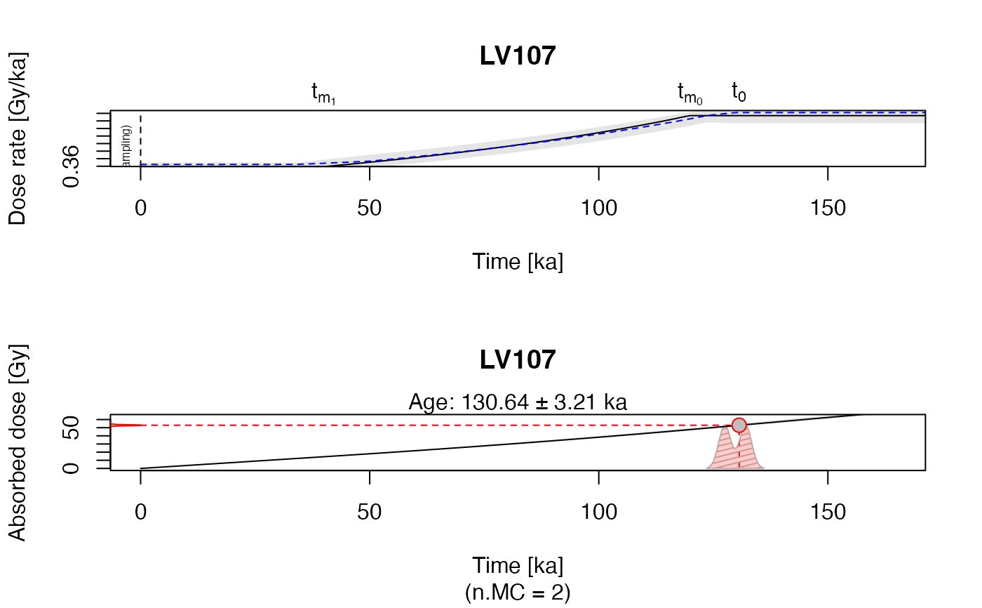
Upper plot: Dose rate evolution over time backwards. The solid black line is the calculation
output, the grey shaded area indicates the 2-sigma error margins. The dashed blue line is an indicator
of the quality of the error estimations based on Monte Carlo (MC) runs.The closer it follows the
black line, the more reliable are the given error margins.
Lower plot: Totally absorbed dose over time. The plot is an representation of the 'new' age based on the carbonate modelling.
Details
This function is the starting point for the dose rate modelling for carbonate enrich
environments. It provides basically the same functionality as the original version of 'Carb', i.e.
you should be also aware of the limitations of this modelling approach. In particular: The model
assumes a linear carbonate mass increase due to post-depositional processes. Please read the
references cited blow.
Uncertainty estimation
For estimating the uncertainties, Monte-Carlo (MC) simulation runs are used. For very
small values (close to 0) this can, however, lead to edge effects (similar in 'Carb') since
values below 0 are set to 0.
How to cite
Kreutzer, S., 2026. model_DoseRate(): Model dose rate evolution in carbonate-rich samples. Function version 0.3.0. In: Kreutzer, S., Nathan, R.P., Mauz, B., 2026. RCarb: Dose Rate Modelling of Carbonate-Rich Samples . R package version 0.1.8. https://r-lum.github.io/RCarb/
References
Mauz, B., Hoffmann, D., 2014. What to do when carbonate replaced water: Carb, the model for estimating the dose rate of carbonate-rich samples. Ancient TL 32, 24-32. doi:10.26034/la.atl.2014.481
Nathan, R.P., Mauz, B., 2008. On the dose-rate estimate of carbonate-rich sediments for trapped charge dating.
Radiation Measurements 43, 14-25. doi:10.1016/j.radmeas.2007.12.012
Further reading
Nathan, R.P., 2010. Numerical modelling of environmental dose rate and its application to trapped-charge dating. DPhil thesis, St Hugh's College, Oxford. https://ora.ox.ac.uk/objects/ora:6421
Zimmerman, D.W., 1971. Thermoluminescent dating using fine grains from pottery. Archaeometry 13, 29–52.doi:10.1111/j.1475-4754.1971.tb00028.x
Author
Sebastian Kreutzer, Institute of Geography, Heidelberg University (Germany); based on 'MATLAB' code given in file Carb_2007a.m of Carb
Examples
##load example data
data("Example_Data", envir = environment())

##run the function for one sample from
##the dataset
model_DoseRate(
data = Example_Data[14,],
n.MC = 2,
multicores = 2)
#>
#> [model_DoseRate()]
#>
#>  Sample ID:		 LV107
#>  Equivalent dose:	 53  ±  2 Gy
#>  Diameter:		 215 µm
#>  MC runs error estim.:	 2
#>  ------------------------------------------------
#>  Age (conv.):		 149.73  ±  0.417  ka
#>  Age (new):		 130.642  ±  6.354  ka
#>
#>  Dose rate (conv.):	 0.354  ±  0.012  Gy/ka
#>  Dose rate (onset):	 0.5  ±  0.02  Gy/ka
#>  Dose rate (final):	 0.361  ±  0.011  Gy/ka
#>  ------------------------------------------------

#>    SAMP_NAME     K   K_X    T  T_X    U  U_X U238 U238_X U234_U238 U234_U238_X
#> 14     LV107 0.073 0.004 0.67 0.02 0.79 0.07    0      0         0           0
#>    WCI WCI_X WCF WCF_X CC CC_X DIAM DIAM_X COSMIC COSMIC_X INTERNAL INTERNAL_X
#> 14  10     2   5     5 60    2  215     35 0.0876   0.0044        0          0
#>    ONSET ONSET_X FINISH FINISH_X DE DE_X AGE_CONV AGE_CONV_X     AGE AGE_X
#> 14   120      10     40       10 53    2   149.73      0.417 130.642 6.354
#>    DR_CONV DR_CONV_X DR_ONSET DR_ONSET_X DR_FINAL DR_FINAL_X n.MC
#> 14   0.354     0.012      0.5       0.02    0.361      0.011    2
#> SAMP_NAME K K_X T T_X U U_X U238 U238_X U234_U238 U234_U238_X
#> 14 LV107 0.073 0.004 0.67 0.02 0.79 0.07 0 0 0 0
#> WCI WCI_X WCF WCF_X CC CC_X DIAM DIAM_X COSMIC COSMIC_X INTERNAL INTERNAL_X
#> 14 10 2 5 5 60 2 215 35 0.0876 0.0044 0 0
#> ONSET ONSET_X FINISH FINISH_X DE DE_X AGE_CONV AGE_CONV_X AGE AGE_X
#> 14 120 10 40 10 53 2 149.73 0.417 130.642 6.354
#> DR_CONV DR_CONV_X DR_ONSET DR_ONSET_X DR_FINAL DR_FINAL_X n.MC
#> 14 0.354 0.012 0.5 0.02 0.361 0.011 2