Analyse fading measurements and returns the fading rate per decade (g-value)
Source:R/analyse_FadingMeasurement.R
analyse_FadingMeasurement.RdThe function analyses fading measurements and returns a fading rate including an error estimation. The function is not limited to standard fading measurements, as can be seen, e.g., Huntley and Lamothe (2001). Additionally, the density of recombination centres (rho') is estimated after Kars et al. (2008).
Arguments
- object
RLum.Analysis, data.frame or list (required): input object with the measurement data. Alternatively, a list containing RLum.Analysis objects or a data.frame with three columns (x = LxTx, y = LxTx error, z = time since irradiation) can be provided. Can also be a wide table, i.e. a data.frame with a number of columns divisible by 3 and where each triplet has the before mentioned column structure.
Note: The input object should solely consists of the curve needed for the data analysis, i.e. only IRSL curves representing Lx (and Tx). If the object originated from an XSYG file, also the irradiation steps must be preserved in the input object.
If data from multiple aliquots are provided, please see the details below with regard to Lx/Tx normalisation. Note: The function assumes that all your measurements are related to one (comparable) sample. If you have to treat independent samples, you have use this function in a loop.
- structure
character (with default): the structure of the measurement data, one of
'Lx'orc('Lx','Tx').- signal_integral
vector (required): vector with channels for the signal integral (e.g.,
1:10). It is not required if adata.framewithLxTxvalues is provided.- background_integral
vector (required): vector with channels for the background integral (e.g.,
90:100). It is not required if adata.framewithLxTxvalues is provided.- integral_input
character (with default): input type for
signal_integral, one of"channel"(default) or"measurement". If set to"measurement", the best matching channels corresponding to the given time range (in seconds) are selected.- t_star
character, function (with default): method for calculating the time elapsed since irradiation if input is not a
data.frame. Options are:'half'(the default),'half_complex, which uses the long equation in Auclair et al. 2003, and'end', which takes the time between irradiation and the measurement step. Alternatively,t_starcan be a function with one parameter which works ont1. For more information see details.t_starhas no effect if the input is a data.frame, because this input comes without irradiation times.- n.MC
integer (with default): number for Monte Carlo runs for the error estimation.
- verbose
logical (with default): enable/disable output to the terminal.
- plot
logical (with default): enable/disable the plot output.
- plot_singlePanels
logical or numeric (with default): enable/disable single plot mode, i.e. one plot window per plot. Alternatively a vector specifying the plot to be drawn, e.g.,
plot_singlePanels = c(3,4)draws only the last two plots in separate windows.- ...
further arguments that can be passed to internally used functions. Supported arguments:
xlab,log,mtext,plot.trend(enable/disable trend blue line), andxlimfor the two first curve plots, andylimfor the fading curve plot. For further plot customization please use the numerical output of the functions for own plots.
Value
An RLum.Results object is returned:
Slot: @data
| OBJECT | TYPE | COMMENT |
fading_results | data.frame | results of the fading measurement in a table |
fit | lm | object returned by the used linear fitting function stats::lm |
rho_prime | data.frame | results of rho' estimation after Kars et al. (2008) |
LxTx_table | data.frame | Lx/Tx table, if curve data had been provided |
irr.times | integer | vector with the irradiation times in seconds |
Slot: @info
| OBJECT | TYPE | COMMENT |
call | call | the original function call |
Details
All provided output corresponds to the \(tc\) value obtained by this analysis. Additionally, the g-value normalised to 2-days is provided in the output object. The output of this function can be passed to the function calc_FadingCorr.
Fitting and error estimation
For the fitting the function stats::lm is used without applying weights. For the
error estimation all input values, except tc, as the precision can be considered as sufficiently
high enough with regard to the underlying problem, are sampled assuming a normal distribution
for each value with the value as the mean and the provided uncertainty as standard deviation.
The options for t_star
t_star = "half"(the default) The calculation follows the simplified version in Auclair et al. (2003), which reads $$t_{star} := t_1 + (t_2 - t_1)/2$$t_star = "half_complex"This option applies the complex function shown in Auclair et al. (2003), which is derived from Aitken (1985) appendix F, equations 9 and 11. It reads $$t_{star} = t0 * 10^[(t_2 \log(t_2/t_0) - t_1 \log(t_1/t_0) - 0.43(t_2 - t_1))/(t_2 - t_1)]$$ where 0.43 = \(1/\ln(10)\). t0, which is an arbitrary constant, is set to 1. Please note that the equation in Auclair et al. (2003) is incorrect insofar that it reads \(10\exp(...)\), where the base should be 10 and not the Euler's number. Here we use the correct version (base 10).t_star = "end"This option uses the simplest possible form fort_starwhich is the time since irradiation without taking into account any addition parameter and it equals t1 in Auclair et al. (2003)t_star = <function>This last option allows you to provide an R function object that works on t1 and gives you all possible freedom. For instance, you may want to define the following functionfun <- function(x) {x^2}, this would square all values of t1, because internally it callsfun(t1). The name of the function does not matter.
Density of recombination centres
The density of recombination centres, expressed by the dimensionless variable rho', is estimated by fitting equation 5 in Kars et al. (2008) to the data. For the fitting the function stats::nls is used without applying weights. For the error estimation the same procedure as for the g-value is applied (see above).
Multiple aliquots & Lx/Tx normalisation
Be aware that this function will always normalise all \(\frac{L_x}{T_x}\)
values by the \(\frac{L_x}{T_x}\) value of the prompt measurement of the
first aliquot. This implicitly assumes that there are no systematic
inter-aliquot variations in the \(\frac{L_x}{T_x}\) values.
If deemed necessary to normalise the \(\frac{L_x}{T_x}\) values of each
aliquot by its individual prompt measurement please do so before running
analyse_FadingMeasurement and provide the already normalised values for
object instead.
Shine-down curve plots Please note that the shine-down curve plots are for information only. As such a maximum of five pause steps are plotted to avoid graphically overloaded plots. However, all pause times are taken into consideration for the analysis.
How to cite
Kreutzer, S., Burow, C., 2026. analyse_FadingMeasurement(): Analyse fading measurements and returns the fading rate per decade (g-value). Function version 0.1.27. In: Kreutzer, S., Burow, C., Dietze, M., Fuchs, M.C., Schmidt, C., Fischer, M., Friedrich, J., Mercier, N., Philippe, A., Riedesel, S., Autzen, M., Mittelstrass, D., Gray, H.J., Galharret, J., Colombo, M., Steinbuch, L., Boer, A.d., Bluszcz, A., 2026. Luminescence: Comprehensive Luminescence Dating Data Analysis. R package version 1.3.0. https://r-lum.github.io/Luminescence/
References
Aitken, M.J., 1985. Thermoluminescence dating, Studies in archaeological science. Academic Press, London, Orlando.
Auclair, M., Lamothe, M., Huot, S., 2003. Measurement of anomalous fading for feldspar IRSL using SAR. Radiation Measurements 37, 487-492. doi:10.1016/S1350-4487(03)00018-0
Huntley, D.J., Lamothe, M., 2001. Ubiquity of anomalous fading in K-feldspars and the measurement
and correction for it in optical dating. Canadian Journal of Earth Sciences 38,
1093-1106. doi: 10.1139/cjes-38-7-1093
Kars, R.H., Wallinga, J., Cohen, K.M., 2008. A new approach towards anomalous fading correction for feldspar IRSL dating-tests on samples in field saturation. Radiation Measurements 43, 786-790. doi:10.1016/j.radmeas.2008.01.021
Author
Sebastian Kreutzer, F2.1 Geophysical Parametrisation/Regionalisation, LIAG - Institute for Applied Geophysics (Germany)
Christoph Burow, University of Cologne (Germany)
, RLum Developer Team
Examples
## load example data (sample UNIL/NB123, see ?ExampleData.Fading)
data("ExampleData.Fading", envir = environment())
##(1) get fading measurement data (here a three column data.frame)
fading_data <- ExampleData.Fading$fading.data$IR50
##(2) run analysis
g_value <- analyse_FadingMeasurement(
fading_data,
plot = TRUE,
verbose = TRUE,
n.MC = 10)
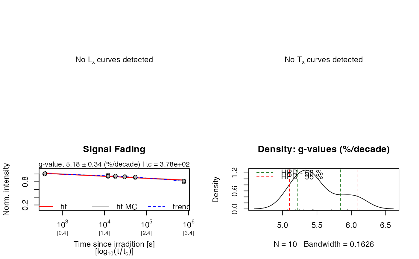 #>
#> [analyse_FadingMeasurement()]
#>
#> n.MC: 10
#> tc: 3.78e+02 s
#> ---------------------------------------------------
#> T_0.5 interpolated: NA
#> T_0.5 predicted: 4e+11
#> g-value: 5.18 ± 1.1 (%/decade)
#> g-value (norm. 2 days): 6.01 ± 1.13 (%/decade)
#> ---------------------------------------------------
#> rho': 3.75e-06 ± 5.43e-07
#> log10(rho'): -5.43 ± 0.06
#> ---------------------------------------------------
##(3) this can be further used in the function
## to correct the age according to Huntley & Lamothe, 2001
results <- calc_FadingCorr(
age.faded = c(100,2),
g_value = g_value,
n.MC = 10)
#>
#>
#> [calc_FadingCorr()]
#>
#> >> Fading correction according to Huntley & Lamothe (2001)
#>
#> .. used g-value: 5.182 ± 1.099 %/decade
#> .. used tc: 1.198e-08 ka
#> .. used kappa: 0.0225 ± 0.0048
#> ----------------------------------------------
#> seed: NA
#> n.MC: 10
#> observations: 10
#> ----------------------------------------------
#> Age (faded): 100 ka ± 2 ka
#> Age (corr.): 203.0812 ka ± 56.8557 ka
#> ----------------------------------------------
#>
#> [analyse_FadingMeasurement()]
#>
#> n.MC: 10
#> tc: 3.78e+02 s
#> ---------------------------------------------------
#> T_0.5 interpolated: NA
#> T_0.5 predicted: 4e+11
#> g-value: 5.18 ± 1.1 (%/decade)
#> g-value (norm. 2 days): 6.01 ± 1.13 (%/decade)
#> ---------------------------------------------------
#> rho': 3.75e-06 ± 5.43e-07
#> log10(rho'): -5.43 ± 0.06
#> ---------------------------------------------------
##(3) this can be further used in the function
## to correct the age according to Huntley & Lamothe, 2001
results <- calc_FadingCorr(
age.faded = c(100,2),
g_value = g_value,
n.MC = 10)
#>
#>
#> [calc_FadingCorr()]
#>
#> >> Fading correction according to Huntley & Lamothe (2001)
#>
#> .. used g-value: 5.182 ± 1.099 %/decade
#> .. used tc: 1.198e-08 ka
#> .. used kappa: 0.0225 ± 0.0048
#> ----------------------------------------------
#> seed: NA
#> n.MC: 10
#> observations: 10
#> ----------------------------------------------
#> Age (faded): 100 ka ± 2 ka
#> Age (corr.): 203.0812 ka ± 56.8557 ka
#> ----------------------------------------------