Calculate the Average Dose and the dose rate dispersion

This functions calculates the Average Dose and their extrinsic dispersion and estimates the standard errors by bootstrapping based on the Average Dose Model by Guerin et al., 2017

calc_AverageDose(
  data,
  sigma_m = NULL,
  Nb_BE = 500,
  na.rm = TRUE,
  plot = TRUE,
  verbose = TRUE,
  ...
)

Arguments

data

RLum.Results or data.frame (required): for data.frame: two columns with De (data[,1]) and De error (values[,2])

sigma_m

numeric (required): the overdispersion resulting from a dose recovery experiment, i.e. when all grains have received the same dose. Indeed in such a case, any overdispersion (i.e. dispersion on top of analytical uncertainties) is, by definition, an unrecognised measurement uncertainty.

Nb_BE

integer (with default): sample size used for the bootstrapping

na.rm

logical (with default): exclude NA values from the data set prior to any further operation.

plot

logical (with default): enables/disables plot output

verbose

logical (with default): enables/disables terminal output

...

further arguments that can be passed to graphics::hist. As three plots are returned all arguments need to be provided as list, e.g., main = list("Plot 1", "Plot 2", "Plot 3"). Note: not all arguments of hist are supported, but the output of hist is returned and can be used of own plots.

Further supported arguments: mtext (character), rug (TRUE/FALSE).

Value

The function returns numerical output and an (optional) plot.

-----------------------------------

[ NUMERICAL OUTPUT ]

-----------------------------------

RLum.Results-object

slot:

@data

[.. $summary : data.frame]

Column	Type	Description
AVERAGE_DOSE	numeric	the obtained average dose
AVERAGE_DOSE.SE	numeric	the average dose error
SIGMA_D	numeric	sigma
SIGMA_D.SE	numeric	standard error of the sigma
IC_AVERAGE_DOSE.LEVEL	character	confidence level average dose
IC_AVERAGE_DOSE.LOWER	character	lower quantile of average dose
IC_AVERAGE_DOSE.UPPER	character	upper quantile of average dose
IC_SIGMA_D.LEVEL	integer	confidence level sigma
IC_SIGMA_D.LOWER	character	lower sigma quantile
IC_SIGMA_D.UPPER	character	upper sigma quantile
L_MAX	character	maximum likelihood value

[.. $dstar : matrix]

Matrix with bootstrap values

[.. $hist : list]

Object as produced by the function histogram

------------------------

[ PLOT OUTPUT ]

------------------------

The function returns two different plot panels.

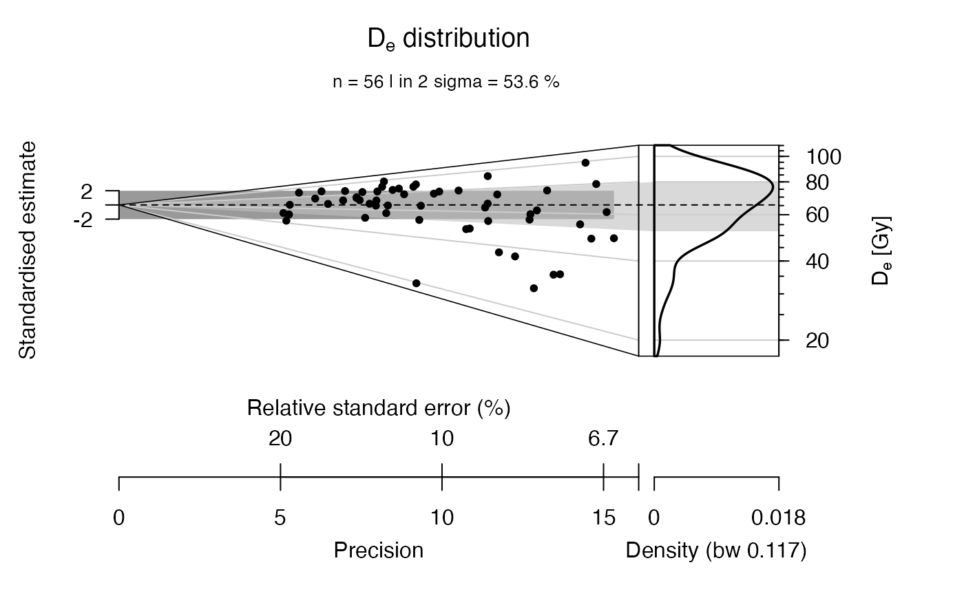
(1) An abanico plot with the dose values

(2) A histogram panel comprising 3 histograms with the equivalent dose and the bootstrapped average dose and the sigma values.

Details

sigma_m

The program requires the input of a known value of sigma_m, which corresponds to the intrinsic overdispersion, as determined by a dose recovery experiment. Then the dispersion in doses (sigma_d) will be that over and above sigma_m (and individual uncertainties sigma_wi).

Note

This function has beta status!

Function version

0.1.5

How to cite

Christophe, C., Philippe, A., Kreutzer, S., 2023. calc_AverageDose(): Calculate the Average Dose and the dose rate dispersion. Function version 0.1.5. In: Kreutzer, S., Burow, C., Dietze, M., Fuchs, M.C., Schmidt, C., Fischer, M., Friedrich, J., Mercier, N., Philippe, A., Riedesel, S., Autzen, M., Mittelstrass, D., Gray, H.J., Galharret, J., 2023. Luminescence: Comprehensive Luminescence Dating Data Analysis. R package version 0.9.23. https://CRAN.R-project.org/package=Luminescence

References

Guerin, G., Christophe, C., Philippe, A., Murray, A.S., Thomsen, K.J., Tribolo, C., Urbanova, P., Jain, M., Guibert, P., Mercier, N., Kreutzer, S., Lahaye, C., 2017. Absorbed dose, equivalent dose, measured dose rates, and implications for OSL age estimates: Introducing the Average Dose Model. Quaternary Geochronology 1-32. doi:10.1016/j.quageo.2017.04.002

Further reading

Efron, B., Tibshirani, R., 1986. Bootstrap Methods for Standard Errors, Confidence Intervals, and Other Measures of Statistical Accuracy. Statistical Science 1, 54-75.

See also

read.table, graphics::hist

Author

Claire Christophe, IRAMAT-CRP2A, Université de Nantes (France), Anne Philippe, Université de Nantes, (France), Guillaume Guérin, IRAMAT-CRP2A, Université Bordeaux Montaigne, (France), Sebastian Kreutzer, Institute of Geography, Heidelberg University (Germany) , RLum Developer Team

Examples

##Example 01 using package example data
##load example data
data(ExampleData.DeValues, envir = environment())

##calculate Average dose
##(use only the first 56 values here)
AD <- calc_AverageDose(ExampleData.DeValues$CA1[1:56,], sigma_m = 0.1)
#> 
#> [calc_AverageDose()]
#> 
#> >> Initialisation <<
#> n:		 56
#> delta:		 65.7939285714286
#> sigma_m:	 0.1
#> sigma_d:	 0.286159381384861
#> 
#> >> Calculation <<
#> log likelihood:	 -19.251
#> confidence intervals
#> --------------------------------------------------
#>                          IC_delta      IC_sigma_d
#> level                        0.95          0.9500
#> CredibleIntervalInf         60.46          0.2175
#> CredibleIntervalSup         70.34          0.3951
#> --------------------------------------------------
#> 
#> >> Results <<
#> ----------------------------------------------------------
#> Average dose:	  65.3597 	se(Aver. dose):	 2.5528
#> sigma_d:	  0.3092 	se(sigma_d):	 0.0476
#> ----------------------------------------------------------


##plot De and set Average dose as central value
plot_AbanicoPlot(
 data = ExampleData.DeValues$CA1[1:56,],
 z.0 = AD$summary$AVERAGE_DOSE)