Luminescence Emission Spectra Deconvolution

Luminescence spectra deconvolution on RLum.Data.Spectrum and matrix objects on an energy scale. The function is optimised for emission spectra typically obtained in the context of TL, OSL and RF measurements detected between 200 and 1000 nm. The function is not prepared to deconvolve TL curves (counts against temperature; no wavelength scale). If you are interested in such analysis, please check, e.g., the package 'tgcd'.

fit_EmissionSpectra(
  object,
  frame = NULL,
  n_components = NULL,
  start_parameters = NULL,
  sub_negative = 0,
  input_scale = NULL,
  method_control = list(),
  verbose = TRUE,
  plot = TRUE,
  ...
)

Arguments

object: RLum.Data.Spectrum, matrix (required): input object. Please note that an energy spectrum is expected
frame: numeric (optional): defines the frame to be analysed
n_components: numeric (optional): allows a number of the aimed number of components. However, it defines rather a maximum than than a minimum. Can be combined with other parameters.
start_parameters: numeric (optional): allows to provide own start parameters for a semi-automated procedure. Parameters need to be provided in eV. Every value provided replaces a value from the automated peak finding algorithm (in ascending order).
sub_negative: numeric (with default): substitute negative values in the input object by the number provided here (default: 0). Can be set to NULL, i.e. negative values are kept.
input_scale: character (optional): defines whether your x-values define wavelength or energy values. For the analysis an energy scale is expected, allowed values are 'wavelength' and 'energy'. If nothing (NULL) is defined, the function tries to understand the input automatically.
method_control: list (optional): options to control the fit method, see details
verbose: logical (with default): enable/disable verbose mode
plot: logical (with default): enable/disable plot output
...: further arguments to be passed to control the plot output (supported: main, xlab, ylab, xlim, ylim, log, mtext, legend (TRUE or FALSE), legend.text, legend.pos)

Value

-----------------------------------

[ NUMERICAL OUTPUT ]

-----------------------------------

RLum.Results-object

slot:

@data

Element	Type	Description
`$data`	`matrix`	the final fit matrix
`$fit`	`nls`	the fit object returned by minpack.lm::nls.lm
`$fit_info`	`list`	a few additional parameters that can be used to asses the quality of the fit

slot:

@info

The original function call

---------------------------------

[ TERMINAL OUTPUT ]

---------------------------------

The terminal output provides brief information on the deconvolution process and the obtained results. Terminal output is only shown of the argument verbose = TRUE.

---------------------------

[ PLOT OUTPUT ]

---------------------------

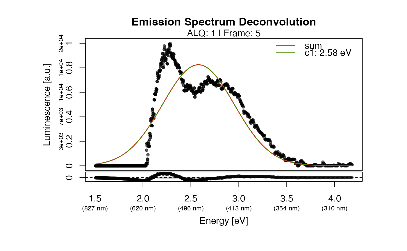
The function returns a plot showing the raw signal with the detected components. If the fitting failed, a basic plot is returned showing the raw data and indicating the peaks detected for the start parameter estimation. The grey band in the residual plot indicates the 10% deviation from 0 (means no residual).

Details

Used equation

The emission spectra (on an energy scale) can be best described as the sum of multiple Gaussian components:

'$$ y = \Sigma Ci * 1/(\sigma_{i} * \sqrt(2 * \pi)) * exp(-1/2 * ((x - \mu_{i})/\sigma_{i}))^2) $$

with the parameters $\sigma$ (peak width) and $\mu$ (peak centre) and $C$ (scaling factor).

Start parameter estimation and fitting algorithm

The spectrum deconvolution consists of the following steps:

Peak finding
Start parameter estimation
Fitting via minpack.lm::nls.lm

The peak finding is realised by an approach (re-)suggested by Petr Pikal via the R-help mailing list (https://stat.ethz.ch/pipermail/r-help/2005-November/thread.html) in November 2005. This goes back to even earlier discussion in 2001 based on Prof Brian Ripley's idea. It smartly uses the functions stats::embed and max.col to identify peaks positions. For the use in this context, the algorithm has been further modified to scale on the input data resolution (cf. source code).

The start parameter estimation uses random sampling from a range of meaningful parameters and repeats the fitting until 1000 successful fits have been produced or the set max.runs value is exceeded.

Currently the best fit is the one with the lowest number for squared residuals, but other parameters are returned as well. If a series of curves needs to be analysed, it is recommended to make few trial runs, then fix the number of components and run at least 10,000 iterations (parameter method_control = list(max.runs = 10000)).

Supported method_control settings

Parameter	Type	Default	Description
`max.runs`	integer	`10000`	maximum allowed search iterations, if exceed the searching stops
`graining`	numeric	`15`	gives control over how coarse or fine the spectrum is split into search intervals for the peak finding algorithm
`norm`	logical	`TRUE`	normalises data to the highest count value before fitting
`trace`	logical	`FALSE`	enables/disables the tracing of the minimisation routine

Function version

0.1.1

Author

Sebastian Kreutzer, Institute of Geography, Heidelberg University (Germany) , RLum Developer Team

How to cite

Kreutzer, S., 2023. fit_EmissionSpectra(): Luminescence Emission Spectra Deconvolution. Function version 0.1.1. In: Kreutzer, S., Burow, C., Dietze, M., Fuchs, M.C., Schmidt, C., Fischer, M., Friedrich, J., Mercier, N., Philippe, A., Riedesel, S., Autzen, M., Mittelstrass, D., Gray, H.J., Galharret, J., 2023. Luminescence: Comprehensive Luminescence Dating Data Analysis. R package version 0.9.23. https://CRAN.R-project.org/package=Luminescence

Examples


##load example data
data(ExampleData.XSYG, envir = environment())

##subtract background
TL.Spectrum@data <- TL.Spectrum@data[] - TL.Spectrum@data[,15]

results <- fit_EmissionSpectra(
 object = TL.Spectrum,
 frame = 5,
 method_control = list(max.runs = 10)
)
#> 
#> [fit_EmissionSpectra()]
#> 
#> >> Treating dataset >> 5 <<
#> >> Wavelength scale detected ...
#> >> Wavelength to energy scale conversion ... 	[OK]
#> 
>> Searching components ... 			[-]
>> Searching components ... 			[/]
>> Searching components ... 			[/]
>> Searching components ... 			[-]
>> Searching components ... 			[-]
>> Searching components ... 			[-]
>> Searching components ... 			[/]
>> Searching components ... 			[/]
>> Searching components ... 			[-]
>> Searching components ... 			[-]
>> Searching components ... 			[OK]
#> 
#> >> Fitting results (1 component model):
#> -------------------------------------------------------------------------
#>            mu      SE(mu)     sigma   SE(sigma)         C      SE(C)
#> [1,] 2.578405 0.006164145 0.3748431 0.005834923 0.7750861 0.01085102
#> -------------------------------------------------------------------------
#> SE: standard error | SSR: 2.164e+01| R^2: 0.807 | R^2_adj: 0.1938
#> (use the output in $fit for a more detailed analysis)
#> 


##deconvolution of a TL spectrum
if (FALSE) {

##load example data

##replace 0 values
results <- fit_EmissionSpectra(
 object = TL.Spectrum,
 frame = 5, main = "TL spectrum"
)

}