Applying a nls-fitting to thermal quenching data.
Arguments
- data
data.frame (required): input data with three columns, the first column contains temperature values in deg. C, columns 2 and 3 the dependent values with its error
- start_param
list (optional): option to provide the start parameters for the fitting, see details
- method_control
list (optional): further options to fine tune the fitting, see details for further information
- n.MC
integer (with default): number of Monte Carlo runs for the error estimation. If
n.MCisNULLor 1, the error estimation is skipped.- verbose
logical (with default): enable/disable output to the terminal.
- plot
logical (with default): enable/disable the plot output.
- ...
further arguments that can be passed to control the plotting, support are
main,pch,col_fit,col_points,lty,lwd,xlab,ylab,xlim,ylim,xaxt
Value
The function returns numerical output and an (optional) plot.
———————————–[ NUMERICAL OUTPUT ]
———————————–
RLum.Results-object
slot: @data
[.. $data : data.frame]
A table with all fitting parameters and the number of Monte Carlo runs used
for the error estimation (this may be smaller that n.MC).
[.. $fit : nls object]
The nls stats::nls object returned by the function minpack.lm::nlsLM. This object can be further passed to other functions supporting an nls object (cf. details section in stats::nls)
slot: @info
[.. $call : call]
The original function call.
———————————–[ GAPHICAL OUTPUT ]
———————————–
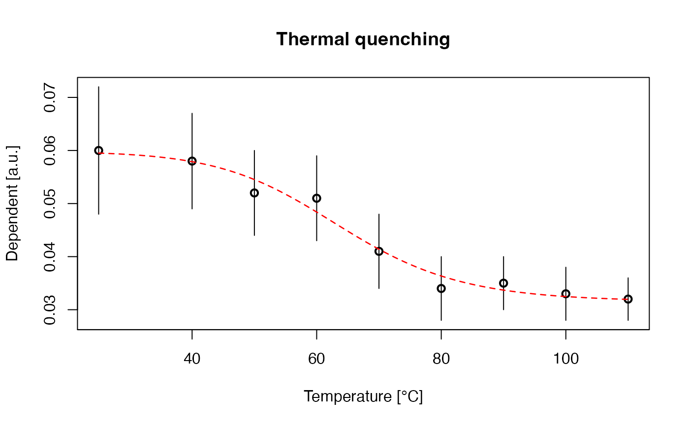
Plotted are temperature against the signal and their uncertainties. The fit is shown as dashed-line (can be modified). Please note that for the fitting the absolute temperature values are used but are re-calculated to deg. C for the plot.
Details
Used equation
The equation used for the fitting is
$$y = A / (1 + C * \exp(-W / (k_B x))) + c$$
W is the energy depth in eV, C is a dimensionless constant, A and c are used to adjust the curve for the given signal, \(k_B\) is the Boltzmann constant in eV/K and x is the absolute temperature in K.
Error estimation
The error estimation is done by varying the input parameters using the given uncertainties in a Monte Carlo simulation. Errors are assumed to follow a normal distribution.
start_param
The function allows the injection of starting values for the parameters to
be optimised via the start_param argument. The parameters must be provided
as a named list.
Examples: start_param = list(A = 1, C = 1e+5, W = 0.5, c = 0)
method_control
The following arguments can be provided via method_control. Please note that arguments provided
via method_control are not further tested, i.e., if the function crashes your input was probably
wrong.
| ARGUMENT | TYPE | DESCRIPTION |
upper | named vector | sets upper fitting boundaries, if provided boundaries for all arguments
are required, e.g., c(A = 0, C = 0, W = 0, c = 0) |
lower | names vector | set lower fitting boundaries (see upper for details) |
trace | logical | enable/disable progression trace for minpack.lm::nlsLM |
weights | numeric | option to provide own weights for the fitting, the length of this
vector needs to be equal to the number for rows of the input data.frame. If set to NULL no weights
are applied. The weights are defined by the third column of the input data.frame. |
How to cite
Kreutzer, S., Colombo, M., 2026. fit_ThermalQuenching(): Fitting Thermal Quenching Data. Function version 0.2. In: Kreutzer, S., Burow, C., Dietze, M., Fuchs, M.C., Schmidt, C., Fischer, M., Friedrich, J., Mercier, N., Philippe, A., Riedesel, S., Autzen, M., Mittelstrass, D., Gray, H.J., Galharret, J., Colombo, M., Steinbuch, L., Boer, A.d., Bluszcz, A., 2026. Luminescence: Comprehensive Luminescence Dating Data Analysis. R package version 1.2.1. https://r-lum.github.io/Luminescence/
References
Wintle, A.G., 1975. Thermal Quenching of Thermoluminescence in Quartz. Geophys. J. R. astr. Soc. 41, 107–113.
Author
Sebastian Kreutzer, F2.1 Geophysical Parametrisation/Regionalisation, LIAG - Institute for Applied Geophysics (Germany)
Marco Colombo, Institute of Geography, Heidelberg University (Germany)
, RLum Developer Team
Examples
##create short example dataset
data <- data.frame(
  T = c(25, 40, 50, 60, 70, 80, 90, 100, 110),
  V = c(0.06, 0.058, 0.052, 0.051, 0.041, 0.034, 0.035, 0.033, 0.032),
  V_X = c(0.012, 0.009, 0.008, 0.008, 0.007, 0.006, 0.005, 0.005, 0.004))

##fit
fit_ThermalQuenching(
 data = data,
 n.MC = NULL)
#>
#> [fit_ThermalQuenching()]
#>
#>  A = 0.02853867 ± NA
#>  C = 3.8315e+14 ± NA
#>  W = 0.9749455 ± NA eV
#>  c = 0.03139589 ± NA
#>  --------------------------------

#>
#>  [RLum.Results-class]
#> 	 originator: fit_ThermalQuenching()
#> 	 data: 2
#>  	 .. $data : data.frame
#> 	 .. $fit : nls
#> 	 additional info elements:  1
#>
#> [RLum.Results-class]
#> originator: fit_ThermalQuenching()
#> data: 2
#> .. $data : data.frame
#> .. $fit : nls
#> additional info elements: 1