Plot filter combinations along with the (optional) net transmission window

The function allows to plot transmission windows for different filters. Missing data for specific wavelengths are automatically interpolated for the given filter data using the function approx. With that a standardised output is reached and a net transmission window can be shown.

plot_FilterCombinations(
  filters,
  wavelength_range = 200:1000,
  show_net_transmission = TRUE,
  interactive = FALSE,
  plot = TRUE,
  ...
)

Arguments

filters: list (required): a named list of filter data for each filter to be shown. The filter data itself should be either provided as data.frame or matrix. (for more options s. Details)
wavelength_range: numeric (with default): wavelength range used for the interpolation
show_net_transmission: logical (with default): show net transmission window as polygon.
interactive: logical (with default): enable/disable interactive plot
plot: logical (with default): enables or disables the plot output
...: further arguments that can be passed to control the plot output. Supported are main, xlab, ylab, xlim, ylim, type, lty, lwd. For non common plotting parameters see the details section.

Value

Returns an S4 object of type RLum.Results.

@data

`Object`	`Type` `Description`	`net_transmission_window`
`matrix`	the resulting net transmission window	`OD_total`
`matrix`	the total optical density	`filter_matrix`

@info

Object Type Description call

Details

Calculations

Net transmission window

The net transmission window of two filters is approximated by

$$T_{final} = T_{1} * T_{2}$$

Optical density

$$OD = -log10(T)$$

Total optical density

$$OD_{total} = OD_{1} + OD_{2}$$

Please consider using own calculations for more precise values.

How to provide input data?

CASE 1

The function expects that all filter values are either of type matrix or data.frame with two columns. The first columns contains the wavelength, the second the relative transmission (but not in percentage, i.e. the maximum transmission can be only become 1).

In this case only the transmission window is show as provided. Changes in filter thickness and reflection factor are not considered.

CASE 2

The filter data itself are provided as list element containing a matrix or data.frame and additional information on the thickness of the filter, e.g., list(filter1 = list(filter_matrix, d = 2)). The given filter data are always considered as standard input and the filter thickness value is taken into account by

$$Transmission = Transmission^(d)$$

with d given in the same dimension as the original filter data.

CASE 3

Same as CASE 2 but additionally a reflection factor P is provided, e.g., list(filter1 = list(filter_matrix, d = 2, P = 0.9)). The final transmission becomes:

$$Transmission = Transmission^(d) * P$$

Advanced plotting parameters

The following further non-common plotting parameters can be passed to the function:

`Argument`	`Datatype`	`Description`
`legend`	`logical`	enable/disable legend
`legend.pos`	`character`	change legend position (graphics::legend)
`legend.text`	`character`	same as the argument `legend` in (graphics::legend)
`net_transmission.col`	`col`	colour of net transmission window polygon
`net_transmission.col_lines`	`col`	colour of net transmission window polygon lines
`net_transmission.density`	`numeric`	specify line density in the transmission polygon
`grid`	`list`	full list of arguments that can be passed to the function graphics::grid

For further modifications standard additional R plot functions are recommend, e.g., the legend can be fully customised by disabling the standard legend and use the function graphics::legend instead.

Function version

0.3.2

Author

Sebastian Kreutzer, Institute of Geography, Heidelberg University (Germany) , RLum Developer Team

How to cite

Kreutzer, S., 2023. plot_FilterCombinations(): Plot filter combinations along with the (optional) net transmission window. Function version 0.3.2. In: Kreutzer, S., Burow, C., Dietze, M., Fuchs, M.C., Schmidt, C., Fischer, M., Friedrich, J., Mercier, N., Philippe, A., Riedesel, S., Autzen, M., Mittelstrass, D., Gray, H.J., Galharret, J., 2023. Luminescence: Comprehensive Luminescence Dating Data Analysis. R package version 0.9.23. https://CRAN.R-project.org/package=Luminescence

Examples


## (For legal reasons no real filter data are provided)

## Create filter sets
filter1 <- density(rnorm(100, mean = 450, sd = 20))
filter1 <- matrix(c(filter1$x, filter1$y/max(filter1$y)), ncol = 2)
filter2 <- matrix(c(200:799,rep(c(0,0.8,0),each = 200)), ncol = 2)

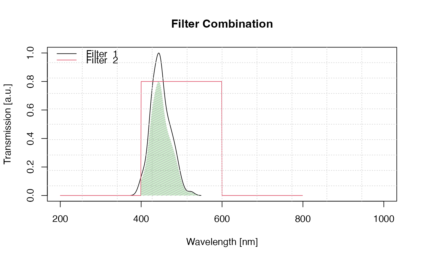
## Example 1 (standard)
plot_FilterCombinations(filters = list(filter1, filter2))


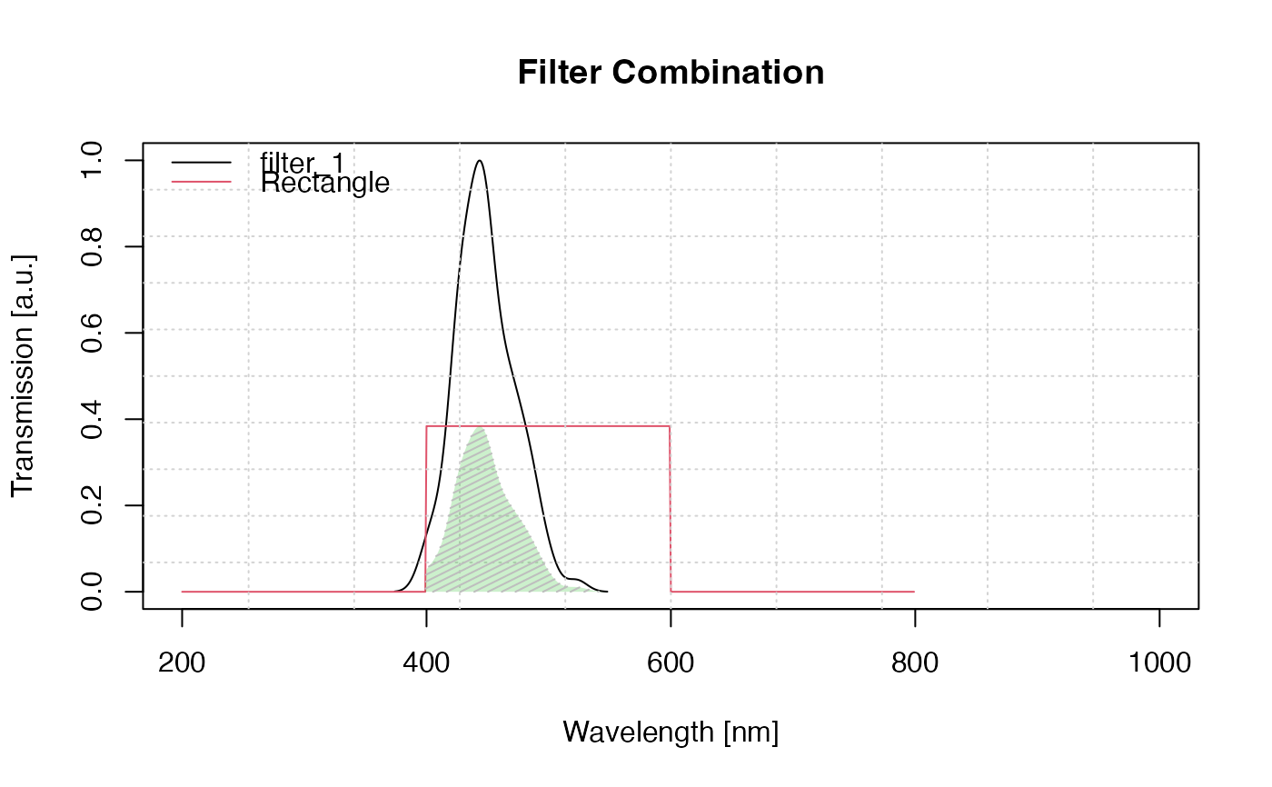
## Example 2 (with d and P value and name for filter 2)
results <- plot_FilterCombinations(
filters = list(filter_1 = filter1, Rectangle = list(filter2, d = 2, P = 0.6)))

results
#> 
#>  [RLum.Results-class]
#> 	 originator: plot_FilterCombinations()
#> 	 data: 3
#>  	 .. $net_transmission_window : matrix
#> 	 .. $OD_total : matrix
#> 	 .. $filter_matrix : matrix
#> 	 additional info elements:  1 

## Example 3 show optical density
plot(results$OD_total)


if (FALSE) {
##Example 4
##show the filters using the interactive mode
plot_FilterCombinations(filters = list(filter1, filter2), interactive = TRUE)

}