Function plots a predefined histogram with an accompanying error plot as suggested by Rex Galbraith at the UK LED in Oxford 2010.
If the normal curve is added, the y-axis in the histogram will show the probability density.
A statistic summary, i.e. a collection of statistic measures of centrality and dispersion (and further measures) can be added by specifying one or more of the following keywords:
"n"(number of samples),"mean"(mean De value),"mean.weighted"(error-weighted mean),"median"(median of the De values),"median.weighted"(error-weighted median),"sdrel"(relative standard deviation in percent),"sdrel.weighted"(error-weighted relative standard deviation in percent),"sdabs"(absolute standard deviation),"sdabs.weighted"(error-weighted absolute standard deviation),"serel"(relative standard error),"serel.weighted"(error-weighted relative standard error),"seabs"(absolute standard error),"seabs.weighted"(error-weighted absolute standard error),"kurtosis"(kurtosis) and"skewness"(skewness).
Usage
plot_Histogram(
  data,
  na.rm = TRUE,
  mtext = "",
  cex.global = 1,
  se = TRUE,
  rug = TRUE,
  normal_curve = FALSE,
  summary = "",
  summary.pos = "sub",
  colour = c("white", "black", "red", "black"),
  interactive = FALSE,
  ...
)
Arguments
- data
data.frame or RLum.Results object (required): for
data.frame: two columns: De (data[,1]) and De error (data[,2]). If the error column is missing or only containsNAvalues, then the error at each measurement is assumed to be 10^-9.- na.rm
logical (with default): excludes
NAvalues from the data set prior to any further operations.- mtext
- cex.global
numeric (with default): global scaling factor.
- se
logical (with default): plots standard error points over the histogram, default is
TRUE.- rug
logical (with default): adds rugs to the histogram, default is
TRUE.- normal_curve
logical (with default): adds a normal curve to the histogram. Mean and standard deviation are calculated from the input data. If
TRUE, the y-axis in the histogram will show the probability density.- summary
character (with default): add statistic measures of centrality and dispersion to the plot. Can be one or more of several keywords. See details for available keywords.
- summary.pos
numeric or character (with default): optional position coordinates or keyword (e.g.
"topright") for the statistical summary. Alternatively, the keyword"sub"may be specified to place the summary below the plot header. However, this latter option in only possible ifmtextis not used. In case of coordinate specification, y-coordinate refers to the right y-axis.- colour
numeric or character (with default): optional vector of length 4 which specifies the colours of the following plot items in exactly this order: histogram bars, rug lines and summary text, normal distribution curve, standard error points (e.g.,
c("grey", "black", "red", "grey")).- interactive
logical (with default): create an interactive histogram plot (requires the 'plotly' package)
- ...
further arguments and graphical parameters passed to plot or hist. If y-axis labels are provided, these must be specified as a vector of length 2 since the plot features two axes (e.g.
ylab = c("axis label 1", "axis label 2")). Y-axes limits (ylim) must be provided as vector of length four, with the first two elements specifying the left axes limits and the latter two elements giving the right axis limits.
Author
Michael Dietze, GFZ Potsdam (Germany)
Sebastian Kreutzer, F2.1 Geophysical Parametrisation/Regionalisation, LIAG - Institute for Applied Geophysics (Germany)
, RLum Developer Team
How to cite
Dietze, M., Kreutzer, S., 2026. plot_Histogram(): Plot a histogram with separate error plot. Function version 0.4.5. In: Kreutzer, S., Burow, C., Dietze, M., Fuchs, M.C., Schmidt, C., Fischer, M., Friedrich, J., Mercier, N., Philippe, A., Riedesel, S., Autzen, M., Mittelstrass, D., Gray, H.J., Galharret, J., Colombo, M., Steinbuch, L., Boer, A.d., Bluszcz, A., 2026. Luminescence: Comprehensive Luminescence Dating Data Analysis. R package version 1.2.1. https://r-lum.github.io/Luminescence/
Examples
## load data
data(ExampleData.DeValues, envir = environment())
ExampleData.DeValues <- convert_Second2Gray(ExampleData.DeValues$BT998,
dose.rate = c(0.0438,0.0019))
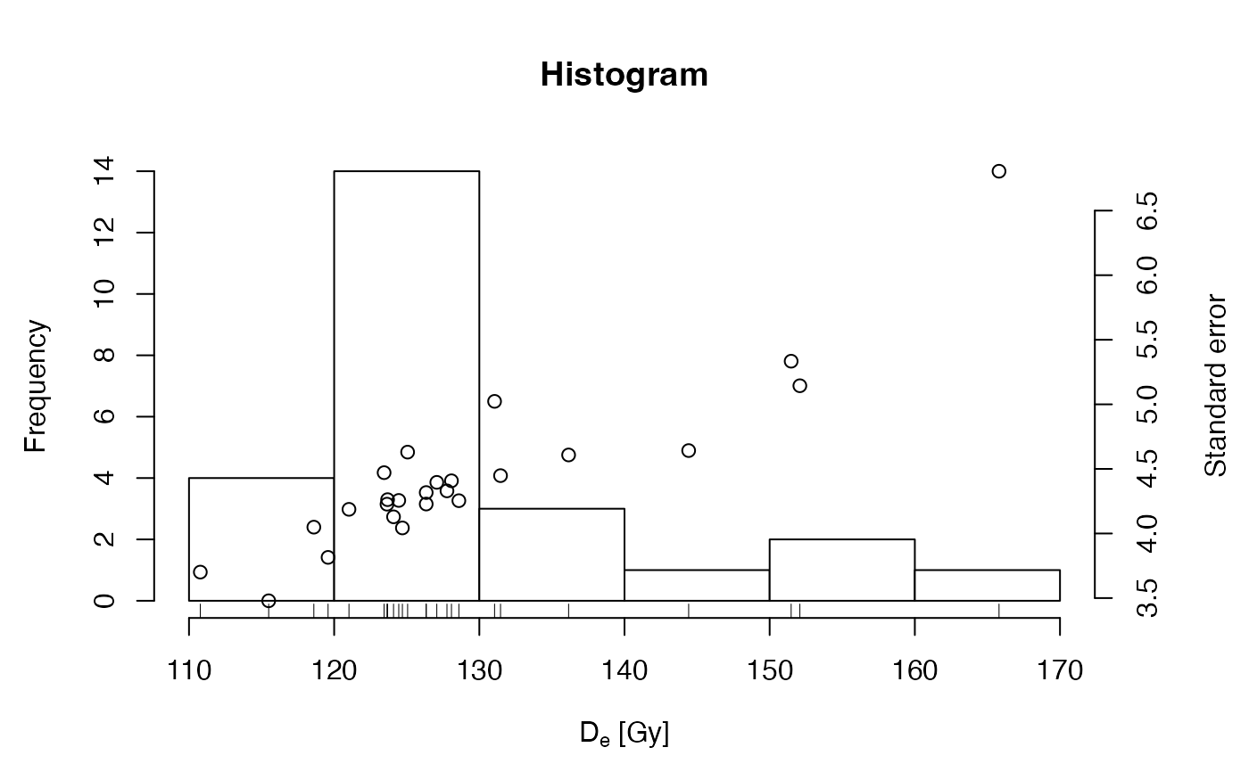
## plot histogram the easiest way
plot_Histogram(ExampleData.DeValues)
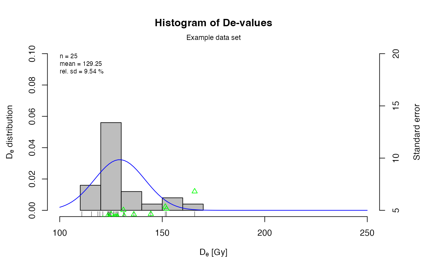
 ## plot histogram with some more modifications
plot_Histogram(ExampleData.DeValues,
rug = TRUE,
normal_curve = TRUE,
cex.global = 0.9,
pch = 2,
colour = c("grey", "black", "blue", "green"),
summary = c("n", "mean", "sdrel"),
summary.pos = "topleft",
main = "Histogram of De-values",
mtext = "Example data set",
ylab = c(expression(paste(D[e], " distribution")),
"Standard error"),
xlim = c(100, 250),
ylim = c(0, 0.1, 5, 20))
## plot histogram with some more modifications
plot_Histogram(ExampleData.DeValues,
rug = TRUE,
normal_curve = TRUE,
cex.global = 0.9,
pch = 2,
colour = c("grey", "black", "blue", "green"),
summary = c("n", "mean", "sdrel"),
summary.pos = "topleft",
main = "Histogram of De-values",
mtext = "Example data set",
ylab = c(expression(paste(D[e], " distribution")),
"Standard error"),
xlim = c(100, 250),
ylim = c(0, 0.1, 5, 20))