Run Monte-Carlo Simulation for LM-OSL (tunnelling transitions)

Runs a Monte-Carlo (MC) simulation of linearly modulated optically stimulated luminescence (LM-OSL) using the tunnelling (TUN) model. Tunnelling refers to quantum mechanical tunnelling processes from the excited state of the trapped charge, into a recombination centre.

run_MC_LM_OSL_TUN(
  A,
  rho,
  times,
  clusters = 10,
  r_c = 0,
  delta.r = 0.1,
  N_e = 200,
  method = "par",
  output = "signal",
  ...
)

Arguments

A

numeric (required): The effective optical excitation rate for the tunnelling process

rho

numeric (required): The dimensionless density of recombination centres (defined as \(\rho\)' in Huntley 2006) (dimensionless)

times

numeric (required): The sequence of time steps within the simulation (s)

clusters

numeric (with default): The number of MC runs

r_c

numeric (with default): Critical distance (>0) that is to be used if the sample has 1 been thermally and/or optically pretreated. This parameter expresses the fact that electron-hole pairs within a critical radius r_c have already been recombined.

delta.r

numeric (with default): Increments of dimensionless distance r'

N_e

numeric (width default): The total number of electron traps available (dimensionless). Can be a vector of length(clusters), shorter values are recycled.

method

character (with default): Sequential 'seq' or parallel 'par'processing. In the parallel mode the function tries to run the simulation on multiple CPU cores (if available) with a positive effect on the computation time.

output

character (with default): output is either the 'signal' (the default) or 'remaining_e' (the remaining charges, electrons, in the trap)

...

further arguments, such as cores to control the number of used CPU cores or verbose to silence the terminal

Value

This function returns an object of class RLumCarlo_Model_Output which is a list consisting of an array with dimension length(times) x length(r) x clusters and a numeric time vector.

Details

The model

$$ I_{TUN}(r',t) = -dn/dt = (A * t/P) * exp(-(\rho')^{-1/3} * r') * n(r',t) $$

Where in the function:
A := the optical excitation rate for the tunnelling process (s^-1)
t := time (s)
P := maximum stimulation time (s)
r' := the dimensionless tunnelling radius
\(\rho\) := rho the dimensionless density of recombination centres see Huntley (2006)
n := the instantaneous number of electrons corresponding to the radius r'

Function version

0.1.0

How to cite

Friedrich, J., Kreutzer, S., 2022. run_MC_LM_OSL_TUN(): Run Monte-Carlo Simulation for LM-OSL (tunnelling transitions). Function version 0.1.0. In: Friedrich, J., Kreutzer, S., Pagonis, V., Schmidt, C., 2022. RLumCarlo: Monte-Carlo Methods for Simulating Luminescence Phenomena. R package version 0.1.9. https://CRAN.R-project.org/package=RLumCarlo

References

Huntley, D.J., 2006. An explanation of the power-law decay of luminescence. Journal of Physics: Condensed Matter, 18(4), 1359.

Pagonis, V. and Kulp, C., 2017. Monte Carlo simulations of tunneling phenomena and nearest neighbor hopping mechanism in feldspars. Journal of Luminescence 181, 114–120. doi:10.1016/j.jlumin.2016.09.014

Pagonis, V., Friedrich, J., Discher, M., Müller-Kirschbaum, A., Schlosser, V., Kreutzer, S., Chen, R. and Schmidt, C., 2019. Excited state luminescence signals from a random distribution of defects: A new Monte Carlo simulation approach for feldspar. Journal of Luminescence 207, 266–272. doi:10.1016/j.jlumin.2018.11.024

Further reading Aitken, M.J., 1985. Thermoluminescence dating. Academic Press.

Jain, M., Guralnik, B., Andersen, M.T., 2012. Stimulated luminescence emission from localized recombination in randomly distributed defects. Journal of Physics: Condensed Matter 24, 385402.

Author

Johannes Friedrich, University of Bayreuth (Germany), Sebastian Kreutzer, Institute of Geography, Heidelberg University (Germany)

Examples

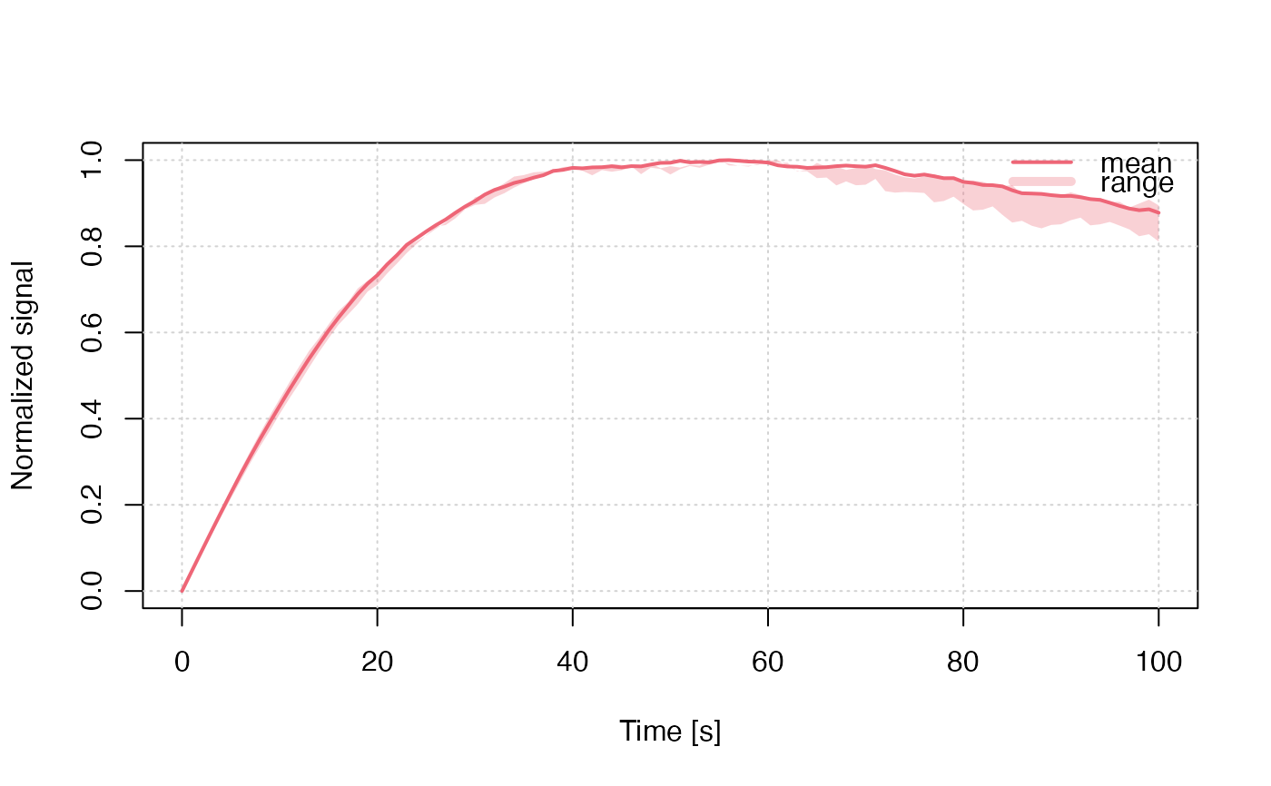
##the short example
run_MC_LM_OSL_TUN(
 A = 1,
 rho = 1e-3,
 times = 0:100,
 clusters = 10,
 N_e = 100,
 r_c = 0.1,
 delta.r = 1e-1,
 method = "seq",
 output = "signal") %>%
plot_RLumCarlo(norm = TRUE)


if (FALSE) {
## the long (meaningful) example
results <- run_MC_LM_OSL_TUN(
 A = 1,
 rho = 1e-3,
 times = 0:1000,
 clusters = 30,
 N_e = 100,
 r_c = 0.1,
 delta.r = 1e-1,
 method = "par",
 output = "signal")

plot_RLumCarlo(results, norm = TRUE)
}