Transform a CW-OSL curve into a pLM-OSL curve via interpolation under linear modulation conditions
Source:R/CW2pLMi.R
CW2pLMi.RdTransforms a conventionally measured continuous-wave (CW) OSL-curve into a pseudo linearly modulated (pLM) curve under linear modulation conditions using the interpolation procedure described by Bos & Wallinga (2012).
Arguments
- values
RLum.Data.Curve or data.frame (required): RLum.Data.Curve or
data.framewith measured curve data of type stimulation time (t) (values[,1]) and measured counts (cts) (values[,2])- P
vector (optional): stimulation time in seconds. If no value is given the optimal value is estimated automatically (see details). Greater values of P produce more points in the rising tail of the curve.
Value
The function returns the same data type as the input data type with the transformed curve values.
RLum.Data.Curve
$CW2pLMi.x.t | : transformed time values |
$CW2pLMi.method | : used method for the production of the new data points |
Details
The complete procedure of the transformation is given in Bos & Wallinga
(2012). The input data.frame consists of two columns: time (t) and
count values (CW(t))
Nomenclature
P = stimulation time (s)
1/P = stimulation rate (1/s)
Internal transformation steps
(1) log(CW-OSL) values
(2) Calculate t' which is the transformed time: $$t' = 1/2*1/P*t^2$$
(3)
Interpolate CW(t'), i.e. use the log(CW(t)) to obtain the count values
for the transformed time (t'). Values beyond min(t) and max(t)
produce NA values.
(4)
Select all values for t' < min(t), i.e. values beyond the time resolution
of t. Select the first two values of the transformed data set which contain
no NA values and use these values for a linear fit using lm.
(5)
Extrapolate values for t' < min(t) based on the previously obtained
fit parameters.
(6) Transform values using $$pLM(t) = t/P*CW(t')$$
(7)
Combine values and truncate all values for t' > max(t)
NOTE:
The number of values for t' < min(t) depends on the stimulation
period (P) and therefore on the stimulation rate 1/P. To avoid the
production of too many artificial data at the raising tail of the determined
pLM curves it is recommended to use the automatic estimation routine for
P, i.e. provide no own value for P.
Note
According to Bos & Wallinga (2012) the number of extrapolated points
should be limited to avoid artificial intensity data. If P is
provided manually and more than two points are extrapolated, a warning
message is returned.
How to cite
Kreutzer, S., 2024. CW2pLMi(): Transform a CW-OSL curve into a pLM-OSL curve via interpolation under linear modulation conditions. Function version 0.3.1. In: Kreutzer, S., Burow, C., Dietze, M., Fuchs, M.C., Schmidt, C., Fischer, M., Friedrich, J., Mercier, N., Philippe, A., Riedesel, S., Autzen, M., Mittelstrass, D., Gray, H.J., Galharret, J., Colombo, M., 2024. Luminescence: Comprehensive Luminescence Dating Data Analysis. R package version 0.9.26. https://r-lum.github.io/Luminescence/
References
Bos, A.J.J. & Wallinga, J., 2012. How to visualize quartz OSL signal components. Radiation Measurements, 47, 752-758.
Further Reading
Bulur, E., 1996. An Alternative Technique For Optically Stimulated Luminescence (OSL) Experiment. Radiation Measurements, 26, 701-709.
Bulur, E., 2000. A simple transformation for converting CW-OSL curves to LM-OSL curves. Radiation Measurements, 32, 141-145.
Author
Sebastian Kreutzer, Institute of Geography, Heidelberg University (Germany)
Based on comments and suggestions from:
Adrie J.J. Bos, Delft University of Technology, The Netherlands
, RLum Developer Team
Examples
##(1)
##load CW-OSL curve data
data(ExampleData.CW_OSL_Curve, envir = environment())

##transform values
values.transformed <- CW2pLMi(ExampleData.CW_OSL_Curve)

##plot
plot(values.transformed$x, values.transformed$y.t, log = "x")


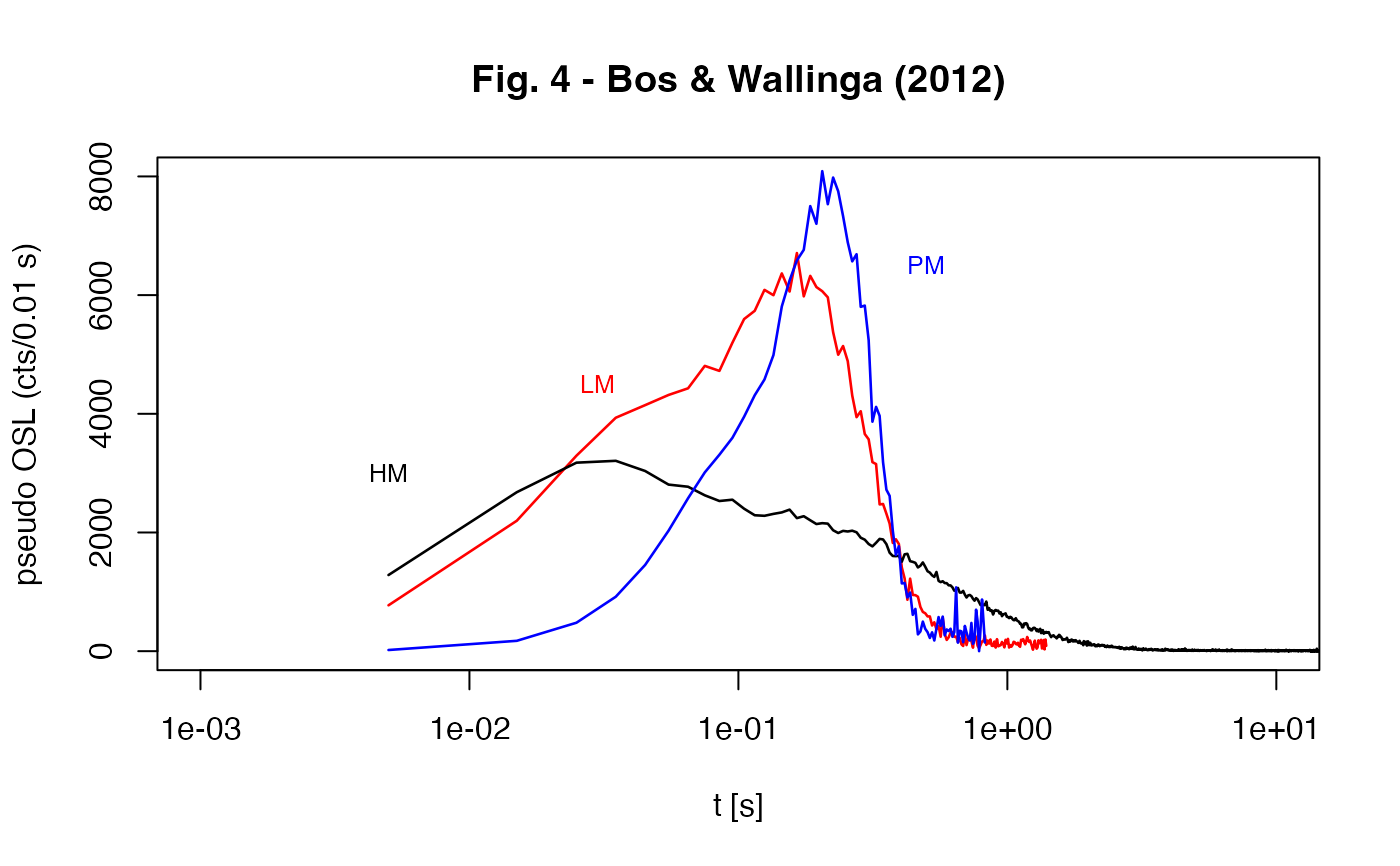
##(2) - produce Fig. 4 from Bos & Wallinga (2012)
##load data
data(ExampleData.CW_OSL_Curve, envir = environment())
values <- CW_Curve.BosWallinga2012

##open plot area
plot(NA, NA,
     xlim = c(0.001,10),
     ylim = c(0,8000),
     ylab = "pseudo OSL (cts/0.01 s)",
     xlab = "t [s]",
     log = "x",
     main = "Fig. 4 - Bos & Wallinga (2012)")


values.t <- CW2pLMi(values, P = 1/20)
lines(values[1:length(values.t[,1]),1],CW2pLMi(values, P = 1/20)[,2],
      col = "red", lwd = 1.3)
text(0.03,4500,"LM", col = "red", cex = .8)

values.t <- CW2pHMi(values, delta = 40)
#> Warning: [CW2pHMi()] 56 values have been found and replaced by the mean of the nearest values
lines(values[1:length(values.t[,1]),1],CW2pHMi(values, delta = 40)[,2],
      col = "black", lwd = 1.3)
#> Warning: [CW2pHMi()] 56 values have been found and replaced by the mean of the nearest values
text(0.005,3000,"HM", cex =.8)

values.t <- CW2pPMi(values, P = 1/10)
#> Warning: t' is beyond the time resolution. Only two data points have been extrapolated, the first 3 points have been set to 0!
lines(values[1:length(values.t[,1]),1], CW2pPMi(values, P = 1/10)[,2],
      col = "blue", lwd = 1.3)
#> Warning: t' is beyond the time resolution. Only two data points have been extrapolated, the first 3 points have been set to 0!
text(0.5,6500,"PM", col = "blue", cex = .8)
