The function determines weighted non-linear least-squares estimates of the
component parameters of an LM-OSL curve (Bulur 1996) for a given number of
components and returns various component parameters. The fitting procedure
uses the Levenberg-Marquardt algorithm as implemented in function nlsLM
from package minpack.lm.
Usage
fit_LMCurve(
  object,
  object.bg,
  n.components = 3,
  start_values = NULL,
  input.dataType = c("LM", "pLM"),
  sample_code = "",
  sample_ID = "",
  LED.power = 36,
  LED.wavelength = 470,
  fit.trace = FALSE,
  fit.calcError = FALSE,
  bg.subtraction = c("polynomial", "linear", "channel", "none"),
  verbose = TRUE,
  plot = TRUE,
  plot.BG = FALSE,
  plot.residuals = TRUE,
  plot.contribution = TRUE,
  legend = TRUE,
  legend.pos = "topright",
  method_control = list(),
  ...
)
Arguments
- object
RLum.Data.Curve or data.frame (required): x,y data of measured values (time and counts).
- object.bg
RLum.Data.Curve or data.frame (optional): x,y data of measured values (time and counts) for background subtraction.
- n.components
integer (with default): fixed number of components that are to be recognised during fitting (min = 1, max = 7).
- start_values
data.frame (optional): starting values for
Imandxmparameters in the fit. If set toNULL, an automatic start value estimation is attempted (see details).- input.dataType
character (with default): alter the plot output depending on the input data:
"LM"or"pLM"(pseudo-LM). See: convert_CW2pLM- sample_code
character (optional): sample code used for the plot and the optional output table (mtext).
- sample_ID
character (optional): additional identifier used as column header for the table output.
- LED.power
numeric (with default): LED power (max.) used for intensity ramping in mW/cm². Note: This value is used for the calculation of the absolute photoionisation cross section.
- LED.wavelength
numeric (with default): LED wavelength in nm used for stimulation. Note: This value is used for the calculation of the absolute photoionisation cross section.
- fit.trace
logical (with default): traces the fitting process on the terminal.
- fit.calcError
logical (with default): calculate 1-sigma error range of components using stats::confint.
- bg.subtraction
character (with default): specifies method for background subtraction (one of
"polynomial","linear","channel", or"none", see Details). Only considered ifobject.bgis specified.- verbose
logical (with default): enable/disable output to the terminal.
- plot
logical (with default): enable/disable the plot output.
- plot.BG
logical (with default): enable/disable a plot of the background values with the fit used for the background subtraction.
- plot.residuals
logical (with default): enable/disable the plot of the residuals.
- plot.contribution
logical (with default): enable/disable the plot of the component contribution.
- legend
logical (with default): enable/disable the plot legend.
- legend.pos
character (with default): keyword specifying the position of the legend.
- method_control
list (optional): options to control the output produced. Currently only the 'export.comp.contrib.matrix' (logical) option is supported, to enable/disable export of the component contribution matrix.
- ...
Further arguments that may be passed to the plot output, e.g.
main,xlab,xlab,xlim,ylim,cex,log.
Value
Various types of plots are returned. For details see above. Furthermore an
RLum.Results object is returned with the following structure:
@data:
.. $data : data.frame with fitting results.. $fit : nls (nls object).. $component_matrix : matrix with numerical xy-values of the single fitted components with the resolution of the input data
.. $component.contribution.matrix : list component distribution matrix
(produced only if method_control$export.comp.contrib.matrix = TRUE)
info:
.. $call : call the original function call
Matrix structure for the distribution matrix:
Column 1 and 2: time and rev(time) values
Additional columns are used for the components, two for each component,
containing I0 and n0. The last columns cont. provide information on
the relative component contribution for each time interval including the row
sum for this values.
Details
Fitting function
The function for the fitting has the general form:
$$y = (\exp(0.5) * Im_1 * x / xm_1) * \exp(-x^2 / (2 * xm_1^2)) + \ldots + \exp(0.5) * Im_i * x / xm_i) * \exp(-x^2 / (2 * xm_i^2))$$
where \(1 < i < 8\)
This function and the equations for the conversion to b (detrapping probability) and n0 (proportional to initially trapped charge) have been taken from Kitis et al. (2008):
$$xm_i=\sqrt{\max(t)/b_i}$$ $$Im_i = \exp(-0.5) n0/xm_i$$
Background subtraction
When a background signal is provided with the object.bg argument, the
user can choose among three methods for background subtraction by setting
the bg.subtraction argument to one of these:
"polynomial"(default): a polynomial function is fitted using glm and the resulting function is used for background subtraction: $$y = a x^4 + b x^3 + c x^2 + d x + e$$"linear": a linear function is fitted using glm and the resulting function is used for background subtraction: $$y = a x + b$$"channel": the measured background signal is subtracted channel-wise from the measured signal."none": this disables background subtraction even ifobject.bgis provided.
Start values
The choice of the initial parameters for the nls-fitting is a crucial
point and the fitting procedure may mainly fail due to ill chosen start
parameters. Here, three options are provided:
(a)
If start_values is not provided by the user, a cheap guess is made
by using the detrapping values found by Jain et al. (2003) for quartz for a
maximum of 7 components. Based on these values, the pseudo start parameters
xm and Im are recalculated for the given data set. In all cases, fitting
starts with the ultra-fast component and (depending on n.components)
steps through the following values. If no fit could be achieved, an error
plot (for plot = TRUE) with the pseudo curve (based on the
pseudo start parameters) is provided. This may give the opportunity to
identify appropriate start parameters visually.
(b) If start values are provided, the function works like a simple nls fitting approach.
Goodness of fit
The goodness of the fit is given by a pseudo-R² value (pseudo coefficient of determination). According to Lave (1970), the value is calculated as:
$$pseudoR^2 = 1 - RSS/TSS$$
where \(RSS\) is the Residual Sum of Squares, and \(TSS\) is the Total Sum of Squares.
Error of fitted component parameters
The 1-sigma error for the components is calculated using the function stats::confint. Due to considerable calculation time, this option is disabled by default. In addition, the error for the components can be estimated by using internal R functions like summary. See the nls help page for more information.
For more details on the nonlinear regression in R, see Ritz & Streibig (2008).
Note
The pseudo-R² may not be the best parameter to describe the goodness
of the fit. The trade off between the n.components and the pseudo-R²
value currently remains unconsidered.
The function does not ensure that the fitting procedure has reached a global minimum rather than a local minimum! In any case of doubt, the use of manual start values is highly recommended.
How to cite
Kreutzer, S., 2026. fit_LMCurve(): Non-linear Least Squares Fit for LM-OSL curves. Function version 0.3.8. In: Kreutzer, S., Burow, C., Dietze, M., Fuchs, M.C., Schmidt, C., Fischer, M., Friedrich, J., Mercier, N., Philippe, A., Riedesel, S., Autzen, M., Mittelstrass, D., Gray, H.J., Galharret, J., Colombo, M., Steinbuch, L., Boer, A.d., Bluszcz, A., 2026. Luminescence: Comprehensive Luminescence Dating Data Analysis. R package version 1.3.0. https://r-lum.github.io/Luminescence/
References
Bulur, E., 1996. An Alternative Technique For Optically Stimulated Luminescence (OSL) Experiment. Radiation Measurements 26, 5, 701-709.
Jain, M., Murray, A.S., Boetter-Jensen, L., 2003. Characterisation of blue-light stimulated luminescence components in different quartz samples: implications for dose measurement. Radiation Measurements 37 (4-5), 441-449.
Kitis, G. & Pagonis, V., 2008. Computerized curve deconvolution analysis for LM-OSL. Radiation Measurements 43, 737-741.
Lave, C.A.T., 1970. The Demand for Urban Mass Transportation. The Review of Economics and Statistics 52 (3), 320-323.
Ritz, C. & Streibig, J.C., 2008. Nonlinear Regression with R. R. Gentleman, K. Hornik, & G. Parmigiani, eds., Springer, p. 150.
Author
Sebastian Kreutzer, F2.1 Geophysical Parametrisation/Regionalisation, LIAG - Institute for Applied Geophysics (Germany) , RLum Developer Team
Examples
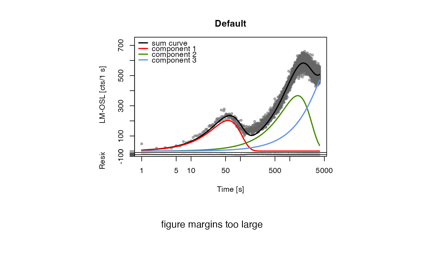
##(1) fit LM data without background subtraction
data(ExampleData.FittingLM, envir = environment())
fit_LMCurve(values.curve, n.components = 3, log = "x")
#>
#> [fit_LMCurve()]
#>
#> Fitting was done using a 3-component function:
#>
#> xm.1 xm.2 xm.3 Im.1 Im.2 Im.3
#> 56.18245 1449.72375 7878.17948 202.76713 367.30183 639.20939
#>
#> (equation used for fitting according to Kitis & Pagonis, 2008)
#> ------------------------------------------------------------------------------
#> (1) Corresponding values according to the equation in Bulur, 1996 for b and n0:
#>
#> b1 = 1.267239e+00 ± NA
#> n01 = 1.878216e+04 ± NA
#>
#> b2 = 1.903222e-03 ± NA
#> n02 = 8.779213e+05 ± NA
#>
#> b3 = 6.444782e-05 ± NA
#> n03 = 8.302641e+06 ± NA
#>
#> cs from component.1 = 1.488e-17 cm^2 >> relative: 1
#> cs from component.2 = 2.234e-20 cm^2 >> relative: 0.0015
#> cs from component.3 = 7.566e-22 cm^2 >> relative: 1e-04
#>
#> (stimulation intensity value used for calculation: 8.517725e+16 1/s 1/cm^2)
#> (errors quoted as 1-sigma uncertainties)
#> ------------------------------------------------------------------------------
#>
#> pseudo-R^2 = 0.9557
 #>
#> [RLum.Results-class]
#> originator: fit_LMCurve()
#> data: 4
#> .. $data : data.frame
#> .. $fit : nls
#> .. $component_matrix : matrix
#> .. $component.contribution.matrix : list
#> additional info elements: 1
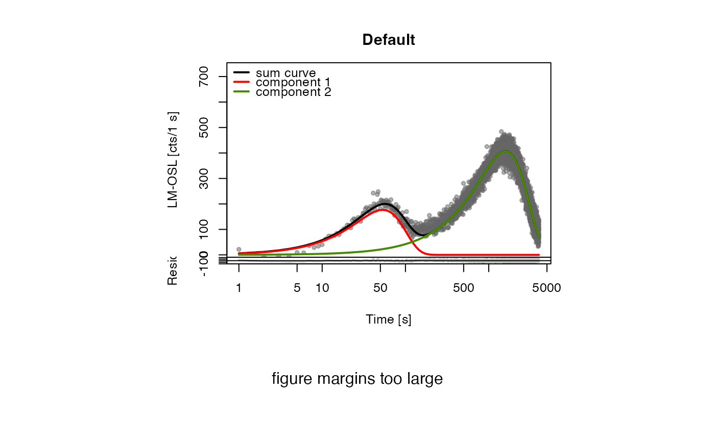
##(2) fit LM data with background subtraction and export as JPEG
## -alter file path for your preferred system
##jpeg(file = "~/Desktop/Fit_Output\%03d.jpg", quality = 100,
## height = 3000, width = 3000, res = 300)
data(ExampleData.FittingLM, envir = environment())
fit_LMCurve(values.curve, object.bg = values.curveBG,
n.components = 2, log = "x", plot.BG = TRUE)
#>
#> [RLum.Results-class]
#> originator: fit_LMCurve()
#> data: 4
#> .. $data : data.frame
#> .. $fit : nls
#> .. $component_matrix : matrix
#> .. $component.contribution.matrix : list
#> additional info elements: 1
##(2) fit LM data with background subtraction and export as JPEG
## -alter file path for your preferred system
##jpeg(file = "~/Desktop/Fit_Output\%03d.jpg", quality = 100,
## height = 3000, width = 3000, res = 300)
data(ExampleData.FittingLM, envir = environment())
fit_LMCurve(values.curve, object.bg = values.curveBG,
n.components = 2, log = "x", plot.BG = TRUE)
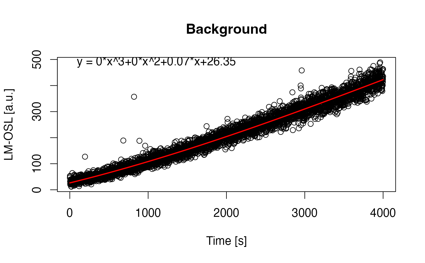 #> [fit_LMCurve()] >> Background subtracted (method = 'polynomial')
#>
#> [fit_LMCurve()]
#>
#> Fitting was done using a 2-component function:
#>
#> xm.1 xm.2 Im.1 Im.2
#> 53.32213 1587.57212 176.74173 406.89921
#>
#> (equation used for fitting according to Kitis & Pagonis, 2008)
#> ------------------------------------------------------------------------------
#> (1) Corresponding values according to the equation in Bulur, 1996 for b and n0:
#>
#> b1 = 1.406841e+00 ± NA
#> n01 = 1.553795e+04 ± NA
#>
#> b2 = 1.587059e-03 ± NA
#> n02 = 1.065044e+06 ± NA
#>
#> cs from component.1 = 1.652e-17 cm^2 >> relative: 1
#> cs from component.2 = 1.863e-20 cm^2 >> relative: 0.0011
#>
#> (stimulation intensity value used for calculation: 8.517725e+16 1/s 1/cm^2)
#> (errors quoted as 1-sigma uncertainties)
#> ------------------------------------------------------------------------------
#>
#> pseudo-R^2 = 0.9417
#> [fit_LMCurve()] >> Background subtracted (method = 'polynomial')
#>
#> [fit_LMCurve()]
#>
#> Fitting was done using a 2-component function:
#>
#> xm.1 xm.2 Im.1 Im.2
#> 53.32213 1587.57212 176.74173 406.89921
#>
#> (equation used for fitting according to Kitis & Pagonis, 2008)
#> ------------------------------------------------------------------------------
#> (1) Corresponding values according to the equation in Bulur, 1996 for b and n0:
#>
#> b1 = 1.406841e+00 ± NA
#> n01 = 1.553795e+04 ± NA
#>
#> b2 = 1.587059e-03 ± NA
#> n02 = 1.065044e+06 ± NA
#>
#> cs from component.1 = 1.652e-17 cm^2 >> relative: 1
#> cs from component.2 = 1.863e-20 cm^2 >> relative: 0.0011
#>
#> (stimulation intensity value used for calculation: 8.517725e+16 1/s 1/cm^2)
#> (errors quoted as 1-sigma uncertainties)
#> ------------------------------------------------------------------------------
#>
#> pseudo-R^2 = 0.9417
 #>
#> [RLum.Results-class]
#> originator: fit_LMCurve()
#> data: 4
#> .. $data : data.frame
#> .. $fit : nls
#> .. $component_matrix : matrix
#> .. $component.contribution.matrix : list
#> additional info elements: 1
##dev.off()
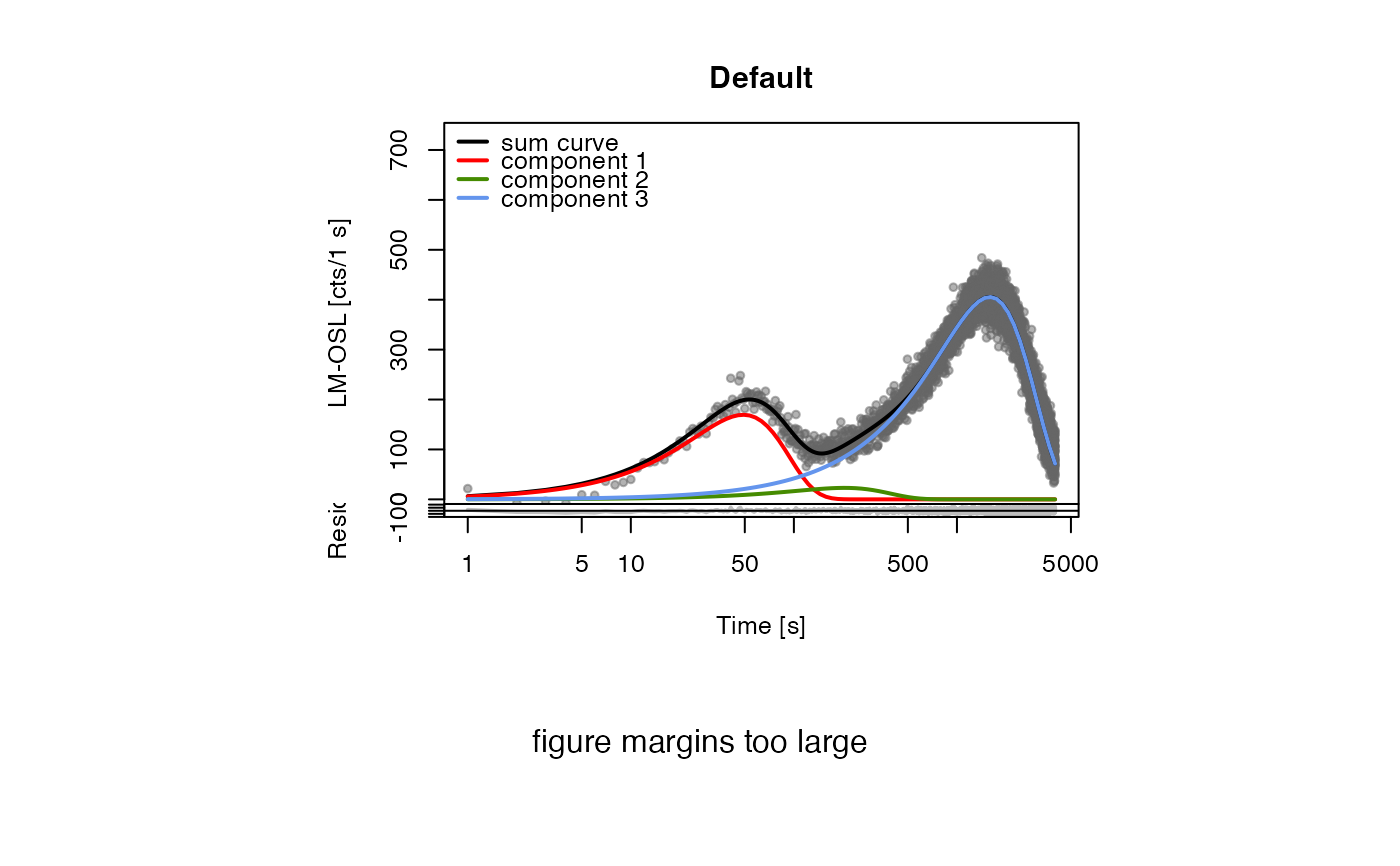
##(3) fit LM data with manual start parameters
data(ExampleData.FittingLM, envir = environment())
fit_LMCurve(values.curve,
object.bg = values.curveBG,
n.components = 3,
log = "x",
start_values = data.frame(Im = c(170,25,400), xm = c(56,200,1500)))
#> [fit_LMCurve()] >> Background subtracted (method = 'polynomial')
#>
#> [fit_LMCurve()]
#>
#> Fitting was done using a 3-component function:
#>
#> xm.1 xm.2 xm.3 Im.1 Im.2 Im.3
#> 49.00545 204.36331 1591.66339 169.43746 23.01060 405.46209
#>
#> (equation used for fitting according to Kitis & Pagonis, 2008)
#> ------------------------------------------------------------------------------
#> (1) Corresponding values according to the equation in Bulur, 1996 for b and n0:
#>
#> b1 = 1.665602e+00 ± NA
#> n01 = 1.368992e+04 ± NA
#>
#> b2 = 9.577543e-02 ± NA
#> n02 = 7.753149e+03 ± NA
#>
#> b3 = 1.578911e-03 ± NA
#> n03 = 1.064017e+06 ± NA
#>
#> cs from component.1 = 1.955e-17 cm^2 >> relative: 1
#> cs from component.2 = 1.124e-18 cm^2 >> relative: 0.0575
#> cs from component.3 = 1.854e-20 cm^2 >> relative: 9e-04
#>
#> (stimulation intensity value used for calculation: 8.517725e+16 1/s 1/cm^2)
#> (errors quoted as 1-sigma uncertainties)
#> ------------------------------------------------------------------------------
#>
#> pseudo-R^2 = 0.9437
#>
#> [RLum.Results-class]
#> originator: fit_LMCurve()
#> data: 4
#> .. $data : data.frame
#> .. $fit : nls
#> .. $component_matrix : matrix
#> .. $component.contribution.matrix : list
#> additional info elements: 1
##dev.off()
##(3) fit LM data with manual start parameters
data(ExampleData.FittingLM, envir = environment())
fit_LMCurve(values.curve,
object.bg = values.curveBG,
n.components = 3,
log = "x",
start_values = data.frame(Im = c(170,25,400), xm = c(56,200,1500)))
#> [fit_LMCurve()] >> Background subtracted (method = 'polynomial')
#>
#> [fit_LMCurve()]
#>
#> Fitting was done using a 3-component function:
#>
#> xm.1 xm.2 xm.3 Im.1 Im.2 Im.3
#> 49.00545 204.36331 1591.66339 169.43746 23.01060 405.46209
#>
#> (equation used for fitting according to Kitis & Pagonis, 2008)
#> ------------------------------------------------------------------------------
#> (1) Corresponding values according to the equation in Bulur, 1996 for b and n0:
#>
#> b1 = 1.665602e+00 ± NA
#> n01 = 1.368992e+04 ± NA
#>
#> b2 = 9.577543e-02 ± NA
#> n02 = 7.753149e+03 ± NA
#>
#> b3 = 1.578911e-03 ± NA
#> n03 = 1.064017e+06 ± NA
#>
#> cs from component.1 = 1.955e-17 cm^2 >> relative: 1
#> cs from component.2 = 1.124e-18 cm^2 >> relative: 0.0575
#> cs from component.3 = 1.854e-20 cm^2 >> relative: 9e-04
#>
#> (stimulation intensity value used for calculation: 8.517725e+16 1/s 1/cm^2)
#> (errors quoted as 1-sigma uncertainties)
#> ------------------------------------------------------------------------------
#>
#> pseudo-R^2 = 0.9437
 #>
#> [RLum.Results-class]
#> originator: fit_LMCurve()
#> data: 4
#> .. $data : data.frame
#> .. $fit : nls
#> .. $component_matrix : matrix
#> .. $component.contribution.matrix : list
#> additional info elements: 1
#>
#> [RLum.Results-class]
#> originator: fit_LMCurve()
#> data: 4
#> .. $data : data.frame
#> .. $fit : nls
#> .. $component_matrix : matrix
#> .. $component.contribution.matrix : list
#> additional info elements: 1