Nonlinear Least Squares Fit for CW-OSL curves -beta version-

The function determines the weighted least-squares estimates of the component parameters of a CW-OSL signal for a given maximum number of components and returns various component parameters. The fitting procedure uses the nls function with the port algorithm.

Fitting function

The function for the CW-OSL fitting has the general form:

$$y = I0_{1}*\lambda_{1}*exp(-\lambda_1*x) + ,\ldots, + I0_{i}*\lambda_{i}*exp(-\lambda_i*x) $$

where $0 < i < 8$

and $\lambda$ is the decay constant
and $I0$ the initial number of trapped electrons.

(for the used equation cf. Boetter-Jensen et al., 2003, Eq. 2.31)

Start values

Start values are estimated automatically by fitting a linear function to the logarithmized input data set. Currently, there is no option to manually provide start parameters.

Goodness of fit

The goodness of the fit is given as pseudoR² value (pseudo coefficient of determination). According to Lave (1970), the value is calculated as:

$$pseudoR^2 = 1 - RSS/TSS$$

where $RSS = Residual~Sum~of~Squares$
and $TSS = Total~Sum~of~Squares$

Error of fitted component parameters

The 1-sigma error for the components is calculated using the function stats::confint. Due to considerable calculation time, this option is deactivated by default. In addition, the error for the components can be estimated by using internal R functions like summary. See the nls help page for more information.

For details on the nonlinear regression in R, see Ritz & Streibig (2008).

Usage

fit_CWCurve(
  values,
  n.components.max,
  fit.failure_threshold = 5,
  fit.method = "port",
  fit.trace = FALSE,
  fit.calcError = FALSE,
  LED.power = 36,
  LED.wavelength = 470,
  cex.global = 0.6,
  sample_code = "Default",
  verbose = TRUE,
  output.terminalAdvanced = TRUE,
  plot = TRUE,
  method_control = list(),
  ...
)

Arguments

values: RLum.Data.Curve or data.frame (required): x, y data of measured values (time and counts). See examples.
n.components.max: vector (optional): maximum number of components that are to be used for fitting. The upper limit is 7.
fit.failure_threshold: integer (with default): limits the failed fitting attempts.
fit.method: character (with default): select fit method, allowed values: 'port' and 'LM'. 'port' uses the 'port' routine from the function nls 'LM' utilises the function nlsLM from the package minpack.lm and with that the Levenberg-Marquardt algorithm.
fit.trace: logical (with default): traces the fitting process on the terminal.
fit.calcError: logical (with default): calculate 1-sigma error range of components using stats::confint
LED.power: numeric (with default): LED power (max.) used for intensity ramping in mW/cm². Note: The value is used for the calculation of the absolute photoionisation cross section.
LED.wavelength: numeric (with default): LED wavelength used for stimulation in nm. Note: The value is used for the calculation of the absolute photoionisation cross section.
cex.global: numeric (with default): global scaling factor.
sample_code: character (optional): sample code used for the plot and the optional output table (mtext).
verbose: logical (with default): enable/disable output to the terminal.
output.terminalAdvanced: logical (with default): enhanced terminal output. Only valid if verbose = TRUE.
plot: logical (with default): enable/disable the plot output.
method_control: list (optional): options to control the output produced. Currently only the 'export.comp.contrib.matrix' (logical) option is supported, to enable/disable export of the component contribution matrix.
...: further arguments and graphical parameters passed to plot.

Value

plot (optional)

the fitted CW-OSL curves are returned as plot.

RLum.Results object

Beside the plot and table output options, an RLum.Results object is returned.

fit: an nls object ($fit) for which generic R functions are provided, e.g. summary, stats::confint, profile. For more details, see nls.

output.table: a data.frame containing the summarised parameters including the error

component.contribution.matrix: matrix containing the values for the component to sum contribution plot ($component.contribution.matrix). Produced only if method_control$export.comp.contrib.matrix = TRUE).

Matrix structure:
Column 1 and 2: time and rev(time) values
Additional columns are used for the components, two for each component, containing I0 and n0. The last columns cont. provide information on the relative component contribution for each time interval including the row sum for this values.

Note

Beta version - This function has not been properly tested yet and should therefore not be used for publication purposes!

The pseudo-R² may not be the best parameter to describe the goodness of the fit. The trade off between the n.components and the pseudo-R² value is currently not considered.

The function does not ensure that the fitting procedure has reached a global minimum rather than a local minimum!

Function version

0.5.4

How to cite

Kreutzer, S., 2025. fit_CWCurve(): Nonlinear Least Squares Fit for CW-OSL curves -beta version-. Function version 0.5.4. In: Kreutzer, S., Burow, C., Dietze, M., Fuchs, M.C., Schmidt, C., Fischer, M., Friedrich, J., Mercier, N., Philippe, A., Riedesel, S., Autzen, M., Mittelstrass, D., Gray, H.J., Galharret, J., Colombo, M., Steinbuch, L., Boer, A.d., 2025. Luminescence: Comprehensive Luminescence Dating Data Analysis. R package version 1.0.1. https://r-lum.github.io/Luminescence/

References

Boetter-Jensen, L., McKeever, S.W.S., Wintle, A.G., 2003. Optically Stimulated Luminescence Dosimetry. Elsevier Science B.V.

Lave, C.A.T., 1970. The Demand for Urban Mass Transportation. The Review of Economics and Statistics, 52 (3), 320-323.

Ritz, C. & Streibig, J.C., 2008. Nonlinear Regression with R. In: R. Gentleman, K. Hornik, G. Parmigiani, eds., Springer, p. 150.

Author

Sebastian Kreutzer, Institute of Geography, Heidelberg University (Germany) , RLum Developer Team

Examples


##load data
data(ExampleData.CW_OSL_Curve, envir = environment())

##fit data
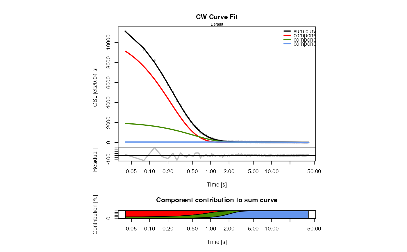
fit <- fit_CWCurve(values = ExampleData.CW_OSL_Curve,
                   main = "CW Curve Fit",
                   n.components.max = 4,
                   log = "x")
#> 
#> [fit_CWCurve()]
#> 
#> Fitting was finally done using a 3-component function (max=4):
#> ------------------------------------------------------------------------------
#> y ~ I0.1 * lambda.1 * exp(-lambda.1 * x) + I0.2 * lambda.2 * exp(-lambda.2 * x) + I0.3 * lambda.3 * exp(-lambda.3 * x)
#> 
#>          I0 I0.error     lambda lambda.error           cs cs.rel
#> c1 2387.620       NA 4.59053773           NA 5.389394e-17 1.0000
#> c2 1053.489       NA 1.95936140           NA 2.300334e-17 0.4268
#> c3 2816.631       NA 0.02054732           NA 2.412301e-19 0.0045
#> ------------------------------------------------------------------------------
#> pseudo-R^2 = 0.9995