Nonlinear Least Squares Fit for OSL surface exposure data
Source:R/fit_SurfaceExposure.R
fit_SurfaceExposure.RdThis function determines the (weighted) least-squares estimates of the parameters of either equation 1 in Sohbati et al. (2012a) or equation 12 in Sohbati et al. (2012b) for a given OSL surface exposure data set (BETA).
Usage
fit_SurfaceExposure(
  data,
  sigmaphi = NULL,
  mu = NULL,
  age = NULL,
  Ddot = NULL,
  D0 = NULL,
  weights = FALSE,
  plot = TRUE,
  legend = TRUE,
  error_bars = TRUE,
  coord_flip = FALSE,
  ...
)
Arguments
- data
data.frame or list (required): Measured OSL surface exposure data with the following structure:
                               (optional)
     | depth (a.u.)| intensity | error |
     |     [ ,1]   |    [ ,2]  | [ ,3] |
     |-------------|-----------|-------|
[1, ]|    ~~~~     |    ~~~~   | ~~~~  |
[2, ]|    ~~~~     |    ~~~~   | ~~~~  |
 ... |     ...     |     ...   |  ...  |
[x, ]|    ~~~~     |    ~~~~   | ~~~~  |
Alternatively, a list of
data.framescan be provided, where eachdata.framehas the same structure as shown above, with the exception that they must not include the optional error column. Providing a list as input automatically activates the global fitting procedure (see details).- sigmaphi
numeric (optional): A numeric value for
sigmaphi, i.e. the charge detrapping rate. Example:sigmaphi = 5e-10- mu
numeric (optional): A numeric value for
mu, i.e. the light attenuation coefficient. Ifdatais a list of n samples, thenmumust be a vector of length 1 or n. Example:mu = 0.9, ormu = c(0.9, 0.8, 0.9).- age
numeric (optional): The age (a) of the sample, if known. If
datais a list of n samples, thenagemust be a numeric vector of length n. Example:age = 10000, orage = c(1e4, 1e5, 1e6).- Ddot
numeric (optional): A numeric value for the environmental dose rate (Gy/ka). For this argument to be considered a value for
D0must also be provided; otherwise it will be ignored.- D0
numeric (optional): A numeric value for the characteristic saturation dose (Gy). For this argument to be considered a value for
Ddotmust also be provided; otherwise it will be ignored.- weights
logical (with default): If
TRUEthe fit will be weighted by the inverse square of the error. Requiresdatato be a data.frame with three columns.- plot
logical (with default): enable/disable the plot output.
- legend
logical (with default): Show or hide the equation inside the plot.
- error_bars
logical (with default): Show or hide error bars (only applies if errors were provided).
- coord_flip
logical (with default): Flip the coordinate system.
- ...
Further parameters passed to plot. Custom parameters include:
Value
Function returns results numerically and graphically:
———————————–[ NUMERICAL OUTPUT ]
———————————–
RLum.Results-object
slot: @data
| Element | Type | Description |
$summary | data.frame | summary of the fitting results |
$data | data.frame | the original input data |
$fit | nls | the fitting object produced by minpack.lm::nlsLM |
$args | character | arguments of the call |
$call | call | the original function call |
slot: @info
Currently unused.
————————[ PLOT OUTPUT ]
————————
A scatter plot of the provided depth-intensity OSL surface exposure data with the fitted model.
Details
Weighted fitting
If weights = TRUE the function will use the inverse square of the error (\(1/\sigma^2\))
as weights during fitting using minpack.lm::nlsLM. Naturally, for this to
take effect individual errors must be provided in the third column of the
data.frame for data. Weighted fitting is not supported if data
is a list of multiple data.frames, i.e., it is not available for global
fitting.
Dose rate
If any of the arguments Ddot or D0 is at its default value (NULL),
this function will fit equation 1 in Sohbati et al. (2012a) to the data. If
the effect of dose rate (i.e., signal saturation) needs to be considered,
numeric values for the dose rate (Ddot) (in Gy/ka) and the characteristic
saturation dose (D0) (in Gy) must be provided. The function will then fit
equation 12 in Sohbati et al. (2012b) to the data.
Note: Currently, this function does not consider the variability
of the dose rate with sample depth (x)! In the original equation the dose
rate D is an arbitrary function of x (term D(x)), but here D is assumed
constant.
Global fitting
If data is list of multiple data.frames, each representing a separate
sample, the function automatically performs a global fit to the data. This
may be useful to better constrain the parameters sigmaphi or mu and
requires that a known age for each sample
(e.g., age = c(100, 1000) if data is a list with two samples).
How to cite
Burow, C., 2026. fit_SurfaceExposure(): Nonlinear Least Squares Fit for OSL surface exposure data. Function version 0.1.0. In: Kreutzer, S., Burow, C., Dietze, M., Fuchs, M.C., Schmidt, C., Fischer, M., Friedrich, J., Mercier, N., Philippe, A., Riedesel, S., Autzen, M., Mittelstrass, D., Gray, H.J., Galharret, J., Colombo, M., Steinbuch, L., Boer, A.d., Bluszcz, A., 2026. Luminescence: Comprehensive Luminescence Dating Data Analysis. R package version 1.3.0. https://r-lum.github.io/Luminescence/
References
Sohbati, R., Murray, A.S., Chapot, M.S., Jain, M., Pederson, J., 2012a. Optically stimulated luminescence (OSL) as a chronometer for surface exposure dating. Journal of Geophysical Research 117, B09202. doi: doi:10.1029/2012JB009383
Sohbati, R., Jain, M., Murray, A.S., 2012b. Surface exposure dating of non-terrestrial bodies using optically stimulated luminescence: A new method. Icarus 221, 160-166.
Examples
## Load example data
data("ExampleData.SurfaceExposure")
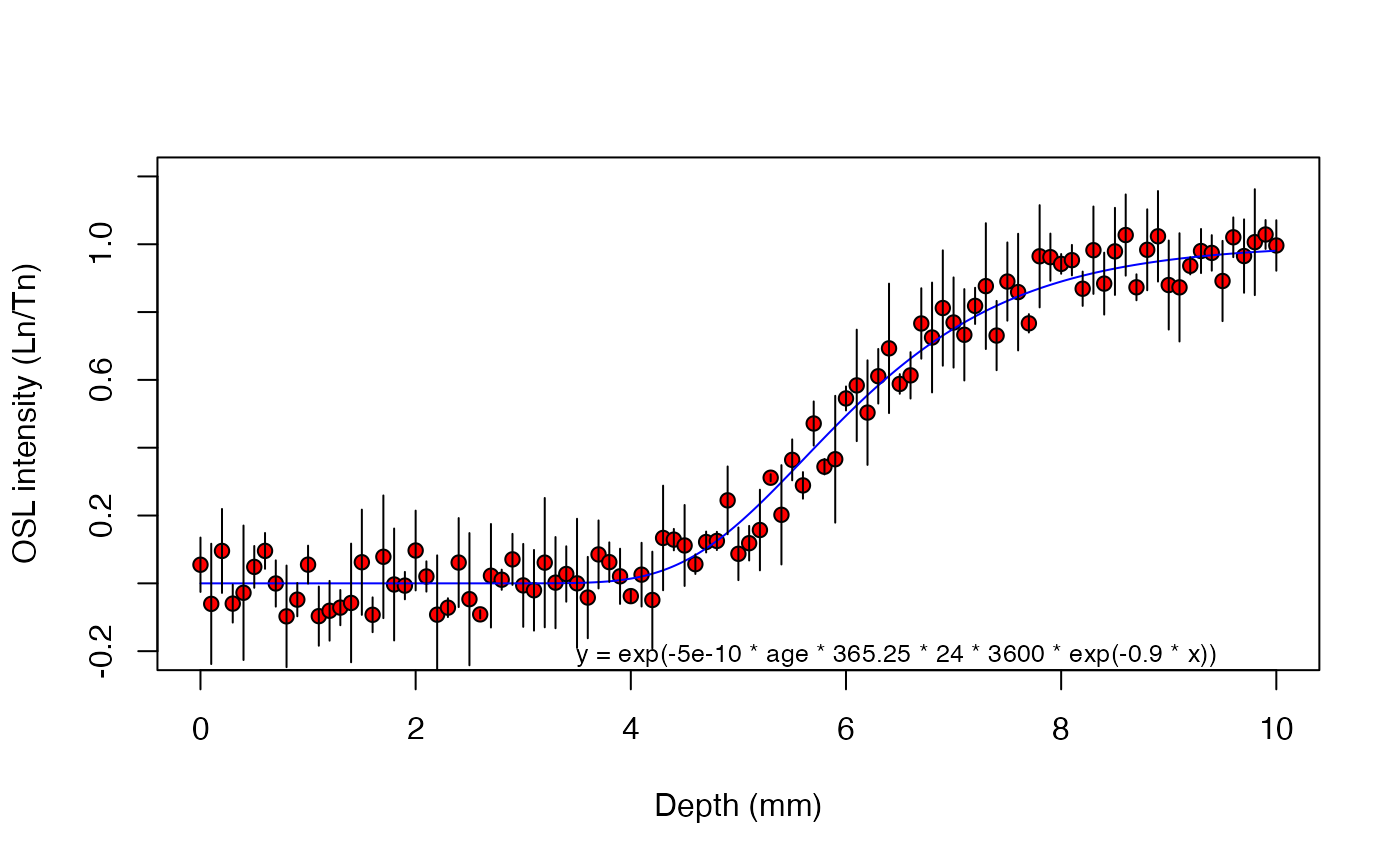
## Example 1 - Single sample
# Known parameters: 10000 a, mu = 0.9, sigmaphi = 5e-10
sample_1 <- ExampleData.SurfaceExposure$sample_1
head(sample_1)
#> depth intensity error
#> 1 0.0 0.05487370 0.08018774
#> 2 0.1 -0.06055516 0.17745452
#> 3 0.2 0.09560277 0.12385804
#> 4 0.3 -0.05973453 0.05593426
#> 5 0.4 -0.02775111 0.19830218
#> 6 0.5 0.04852239 0.06168570
results <- fit_SurfaceExposure(
data = sample_1,
mu = 0.9,
sigmaphi = 5e-10)
 #>
#> [fit_SurfaceExposure()]
#>
#> Estimated parameter(s):
#> ---------------------
#> age (a): 9890 ± 369
#>
#> Fixed parameter(s):
#> -------------------
#> sigmaphi: 5e-10
#> mu: 0.9
#>
get_RLum(results)
#> age age_error sigmaphi sigmaphi_error mu mu_error
#> 1 9892.927 369.0142 5e-10 NA 0.9 NA
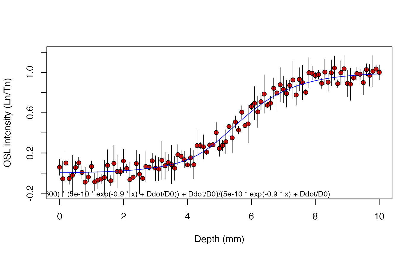
## Example 2 - Single sample and considering dose rate
# Known parameters: 10000 a, mu = 0.9, sigmaphi = 5e-10,
# dose rate = 2.5 Gy/ka, D0 = 40 Gy
sample_2 <- ExampleData.SurfaceExposure$sample_2
head(sample_2)
#> depth intensity error
#> 1 0.0 0.05881908 0.08018774
#> 2 0.1 -0.05623983 0.17745452
#> 3 0.2 0.10032258 0.12385804
#> 4 0.3 -0.05457253 0.05593426
#> 5 0.4 -0.02210573 0.19830218
#> 6 0.5 0.05469614 0.06168570
results <- fit_SurfaceExposure(
data = sample_2,
mu = 0.9,
sigmaphi = 5e-10,
Ddot = 2.5,
D0 = 40)
#>
#> [fit_SurfaceExposure()]
#>
#> Estimated parameter(s):
#> ---------------------
#> age (a): 9890 ± 369
#>
#> Fixed parameter(s):
#> -------------------
#> sigmaphi: 5e-10
#> mu: 0.9
#>
get_RLum(results)
#> age age_error sigmaphi sigmaphi_error mu mu_error
#> 1 9892.927 369.0142 5e-10 NA 0.9 NA
## Example 2 - Single sample and considering dose rate
# Known parameters: 10000 a, mu = 0.9, sigmaphi = 5e-10,
# dose rate = 2.5 Gy/ka, D0 = 40 Gy
sample_2 <- ExampleData.SurfaceExposure$sample_2
head(sample_2)
#> depth intensity error
#> 1 0.0 0.05881908 0.08018774
#> 2 0.1 -0.05623983 0.17745452
#> 3 0.2 0.10032258 0.12385804
#> 4 0.3 -0.05457253 0.05593426
#> 5 0.4 -0.02210573 0.19830218
#> 6 0.5 0.05469614 0.06168570
results <- fit_SurfaceExposure(
data = sample_2,
mu = 0.9,
sigmaphi = 5e-10,
Ddot = 2.5,
D0 = 40)
 #>
#> [fit_SurfaceExposure()]
#>
#> Estimated parameter(s):
#> ---------------------
#> age (a): 9800 ± 675
#>
#> Fixed parameter(s):
#> -------------------
#> sigmaphi: 5e-10
#> mu: 0.9
#>
get_RLum(results)
#> age age_error sigmaphi sigmaphi_error mu mu_error
#> 1 9803.815 674.8718 5e-10 NA 0.9 NA
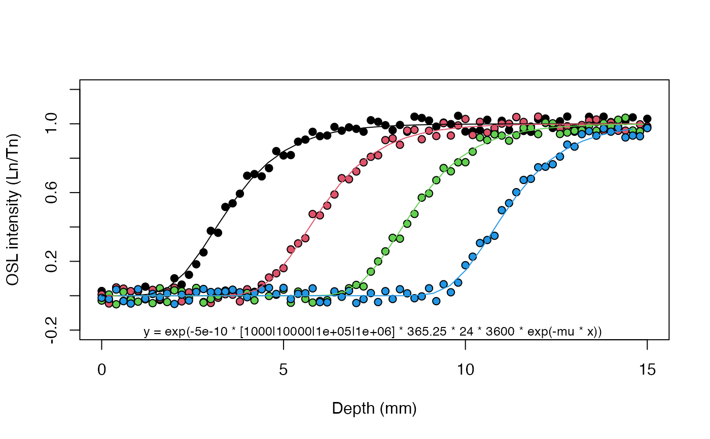
## Example 3 - Multiple samples (global fit) to better constrain 'mu'
# Known parameters: ages = 1e3, 1e4, 1e5, 1e6 a, mu = 0.9, sigmaphi = 5e-10
set_1 <- ExampleData.SurfaceExposure$set_1
str(set_1, max.level = 2)
#> List of 4
#> $ :'data.frame': 76 obs. of 2 variables:
#> ..$ depth : num [1:76] 0 0.2 0.4 0.6 0.8 1 1.2 1.4 1.6 1.8 ...
#> ..$ intensity: num [1:76] 0.0274 -0.0303 0.0478 -0.0298 -0.0134 ...
#> $ :'data.frame': 76 obs. of 2 variables:
#> ..$ depth : num [1:76] 0 0.2 0.4 0.6 0.8 1 1.2 1.4 1.6 1.8 ...
#> ..$ intensity: num [1:76] 0.00714 -0.04511 0.04804 0.04145 0.0266 ...
#> $ :'data.frame': 76 obs. of 2 variables:
#> ..$ depth : num [1:76] 0 0.2 0.4 0.6 0.8 1 1.2 1.4 1.6 1.8 ...
#> ..$ intensity: num [1:76] -0.0284 0.00732 -0.04984 0.02182 -0.02349 ...
#> $ :'data.frame': 76 obs. of 2 variables:
#> ..$ depth : num [1:76] 0 0.2 0.4 0.6 0.8 1 1.2 1.4 1.6 1.8 ...
#> ..$ intensity: num [1:76] -0.0122 -0.0189 0.0358 -0.0314 -0.0454 ...
results <- fit_SurfaceExposure(
data = set_1,
age = c(1e3, 1e4, 1e5, 1e6),
sigmaphi = 5e-10)
#>
#> [fit_SurfaceExposure()]
#>
#> Estimated parameter(s):
#> ---------------------
#> age (a): 9800 ± 675
#>
#> Fixed parameter(s):
#> -------------------
#> sigmaphi: 5e-10
#> mu: 0.9
#>
get_RLum(results)
#> age age_error sigmaphi sigmaphi_error mu mu_error
#> 1 9803.815 674.8718 5e-10 NA 0.9 NA
## Example 3 - Multiple samples (global fit) to better constrain 'mu'
# Known parameters: ages = 1e3, 1e4, 1e5, 1e6 a, mu = 0.9, sigmaphi = 5e-10
set_1 <- ExampleData.SurfaceExposure$set_1
str(set_1, max.level = 2)
#> List of 4
#> $ :'data.frame': 76 obs. of 2 variables:
#> ..$ depth : num [1:76] 0 0.2 0.4 0.6 0.8 1 1.2 1.4 1.6 1.8 ...
#> ..$ intensity: num [1:76] 0.0274 -0.0303 0.0478 -0.0298 -0.0134 ...
#> $ :'data.frame': 76 obs. of 2 variables:
#> ..$ depth : num [1:76] 0 0.2 0.4 0.6 0.8 1 1.2 1.4 1.6 1.8 ...
#> ..$ intensity: num [1:76] 0.00714 -0.04511 0.04804 0.04145 0.0266 ...
#> $ :'data.frame': 76 obs. of 2 variables:
#> ..$ depth : num [1:76] 0 0.2 0.4 0.6 0.8 1 1.2 1.4 1.6 1.8 ...
#> ..$ intensity: num [1:76] -0.0284 0.00732 -0.04984 0.02182 -0.02349 ...
#> $ :'data.frame': 76 obs. of 2 variables:
#> ..$ depth : num [1:76] 0 0.2 0.4 0.6 0.8 1 1.2 1.4 1.6 1.8 ...
#> ..$ intensity: num [1:76] -0.0122 -0.0189 0.0358 -0.0314 -0.0454 ...
results <- fit_SurfaceExposure(
data = set_1,
age = c(1e3, 1e4, 1e5, 1e6),
sigmaphi = 5e-10)
 #>
#> [fit_SurfaceExposure()]
#>
#> Shared estimated parameter(s):
#> ---------------------
#> mu: 0.901 ± 0.00161
#>
#> Fixed parameter(s):
#> -------------------
#> age (a): 1000, 10000, 1e+05, 1e+06
#> sigmaphi: 5e-10
#>
#> To apply the estimated parameters to a sample of unknown age run:
#>
#> fit_SurfaceExposure(data = set_1, sigmaphi = 5e-10, mu = c(0.901, 0.901, 0.901, 0.901))
get_RLum(results)
#> age age_error sigmaphi sigmaphi_error mu mu_error
#> 1 1e+03 NA 5e-10 NA 0.9009494 0.001612274
#> 2 1e+04 NA 5e-10 NA 0.9009494 0.001612274
#> 3 1e+05 NA 5e-10 NA 0.9009494 0.001612274
#> 4 1e+06 NA 5e-10 NA 0.9009494 0.001612274
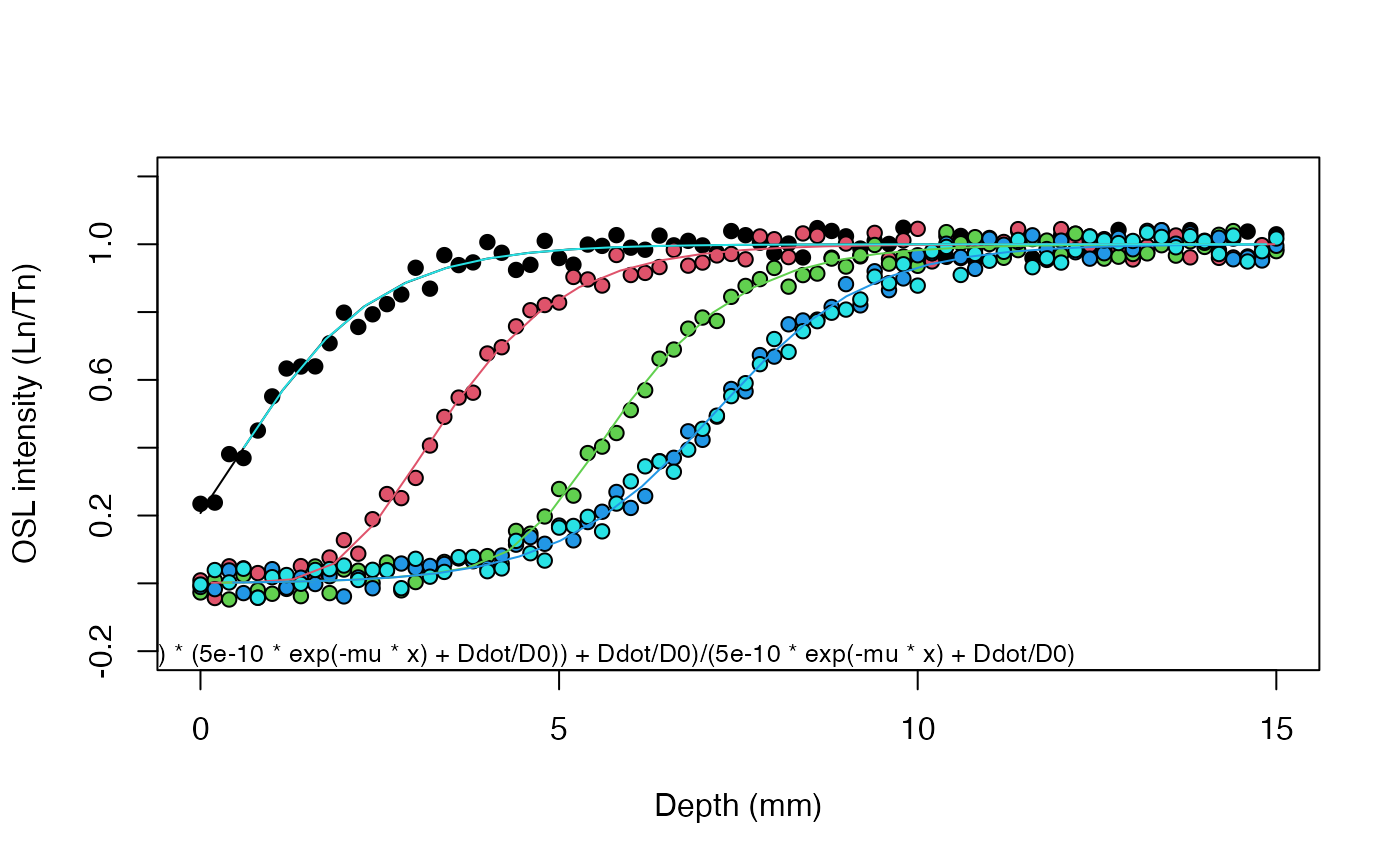
## Example 4 - Multiple samples (global fit) and considering dose rate
# Known parameters: ages = 1e2, 1e3, 1e4, 1e5, 1e6 a, mu = 0.9, sigmaphi = 5e-10,
# dose rate = 1.0 Ga/ka, D0 = 40 Gy
set_2 <- ExampleData.SurfaceExposure$set_2
str(set_2, max.level = 2)
#> List of 5
#> $ :'data.frame': 76 obs. of 2 variables:
#> ..$ depth : num [1:76] 0 0.2 0.4 0.6 0.8 1 1.2 1.4 1.6 1.8 ...
#> ..$ intensity: num [1:76] 0.235 0.238 0.381 0.369 0.451 ...
#> $ :'data.frame': 76 obs. of 2 variables:
#> ..$ depth : num [1:76] 0 0.2 0.4 0.6 0.8 1 1.2 1.4 1.6 1.8 ...
#> ..$ intensity: num [1:76] 0.00872 -0.04321 0.05032 0.04426 0.03029 ...
#> $ :'data.frame': 76 obs. of 2 variables:
#> ..$ depth : num [1:76] 0 0.2 0.4 0.6 0.8 1 1.2 1.4 1.6 1.8 ...
#> ..$ intensity: num [1:76] -0.02682 0.00921 -0.04757 0.02453 -0.02024 ...
#> $ :'data.frame': 76 obs. of 2 variables:
#> ..$ depth : num [1:76] 0 0.2 0.4 0.6 0.8 1 1.2 1.4 1.6 1.8 ...
#> ..$ intensity: num [1:76] -0.0106 -0.0171 0.0381 -0.0287 -0.0422 ...
#> $ :'data.frame': 76 obs. of 2 variables:
#> ..$ depth : num [1:76] 0 0.2 0.4 0.6 0.8 1 1.2 1.4 1.6 1.8 ...
#> ..$ intensity: num [1:76] -0.00358 0.03918 0.00275 0.04301 -0.04237 ...
results <- fit_SurfaceExposure(
data = set_2,
age = c(1e2, 1e3, 1e4, 1e5, 1e6),
sigmaphi = 5e-10,
Ddot = 1,
D0 = 40)
#>
#> [fit_SurfaceExposure()]
#>
#> Shared estimated parameter(s):
#> ---------------------
#> mu: 0.901 ± 0.00161
#>
#> Fixed parameter(s):
#> -------------------
#> age (a): 1000, 10000, 1e+05, 1e+06
#> sigmaphi: 5e-10
#>
#> To apply the estimated parameters to a sample of unknown age run:
#>
#> fit_SurfaceExposure(data = set_1, sigmaphi = 5e-10, mu = c(0.901, 0.901, 0.901, 0.901))
get_RLum(results)
#> age age_error sigmaphi sigmaphi_error mu mu_error
#> 1 1e+03 NA 5e-10 NA 0.9009494 0.001612274
#> 2 1e+04 NA 5e-10 NA 0.9009494 0.001612274
#> 3 1e+05 NA 5e-10 NA 0.9009494 0.001612274
#> 4 1e+06 NA 5e-10 NA 0.9009494 0.001612274
## Example 4 - Multiple samples (global fit) and considering dose rate
# Known parameters: ages = 1e2, 1e3, 1e4, 1e5, 1e6 a, mu = 0.9, sigmaphi = 5e-10,
# dose rate = 1.0 Ga/ka, D0 = 40 Gy
set_2 <- ExampleData.SurfaceExposure$set_2
str(set_2, max.level = 2)
#> List of 5
#> $ :'data.frame': 76 obs. of 2 variables:
#> ..$ depth : num [1:76] 0 0.2 0.4 0.6 0.8 1 1.2 1.4 1.6 1.8 ...
#> ..$ intensity: num [1:76] 0.235 0.238 0.381 0.369 0.451 ...
#> $ :'data.frame': 76 obs. of 2 variables:
#> ..$ depth : num [1:76] 0 0.2 0.4 0.6 0.8 1 1.2 1.4 1.6 1.8 ...
#> ..$ intensity: num [1:76] 0.00872 -0.04321 0.05032 0.04426 0.03029 ...
#> $ :'data.frame': 76 obs. of 2 variables:
#> ..$ depth : num [1:76] 0 0.2 0.4 0.6 0.8 1 1.2 1.4 1.6 1.8 ...
#> ..$ intensity: num [1:76] -0.02682 0.00921 -0.04757 0.02453 -0.02024 ...
#> $ :'data.frame': 76 obs. of 2 variables:
#> ..$ depth : num [1:76] 0 0.2 0.4 0.6 0.8 1 1.2 1.4 1.6 1.8 ...
#> ..$ intensity: num [1:76] -0.0106 -0.0171 0.0381 -0.0287 -0.0422 ...
#> $ :'data.frame': 76 obs. of 2 variables:
#> ..$ depth : num [1:76] 0 0.2 0.4 0.6 0.8 1 1.2 1.4 1.6 1.8 ...
#> ..$ intensity: num [1:76] -0.00358 0.03918 0.00275 0.04301 -0.04237 ...
results <- fit_SurfaceExposure(
data = set_2,
age = c(1e2, 1e3, 1e4, 1e5, 1e6),
sigmaphi = 5e-10,
Ddot = 1,
D0 = 40)
 #>
#> [fit_SurfaceExposure()]
#>
#> Shared estimated parameter(s):
#> ---------------------
#> mu: 0.899 ± 0.00232
#>
#> Fixed parameter(s):
#> -------------------
#> age (a): 100, 1000, 10000, 1e+05, 1e+06
#> sigmaphi: 5e-10
#>
#> To apply the estimated parameters to a sample of unknown age run:
#>
#> fit_SurfaceExposure(data = set_2, sigmaphi = 5e-10, mu = c(0.899, 0.899, 0.899, 0.899, 0.899))
get_RLum(results)
#> age age_error sigmaphi sigmaphi_error mu mu_error
#> 1 1e+02 NA 5e-10 NA 0.8986586 0.002323746
#> 2 1e+03 NA 5e-10 NA 0.8986586 0.002323746
#> 3 1e+04 NA 5e-10 NA 0.8986586 0.002323746
#> 4 1e+05 NA 5e-10 NA 0.8986586 0.002323746
#> 5 1e+06 NA 5e-10 NA 0.8986586 0.002323746
#>
#> [fit_SurfaceExposure()]
#>
#> Shared estimated parameter(s):
#> ---------------------
#> mu: 0.899 ± 0.00232
#>
#> Fixed parameter(s):
#> -------------------
#> age (a): 100, 1000, 10000, 1e+05, 1e+06
#> sigmaphi: 5e-10
#>
#> To apply the estimated parameters to a sample of unknown age run:
#>
#> fit_SurfaceExposure(data = set_2, sigmaphi = 5e-10, mu = c(0.899, 0.899, 0.899, 0.899, 0.899))
get_RLum(results)
#> age age_error sigmaphi sigmaphi_error mu mu_error
#> 1 1e+02 NA 5e-10 NA 0.8986586 0.002323746
#> 2 1e+03 NA 5e-10 NA 0.8986586 0.002323746
#> 3 1e+04 NA 5e-10 NA 0.8986586 0.002323746
#> 4 1e+05 NA 5e-10 NA 0.8986586 0.002323746
#> 5 1e+06 NA 5e-10 NA 0.8986586 0.002323746