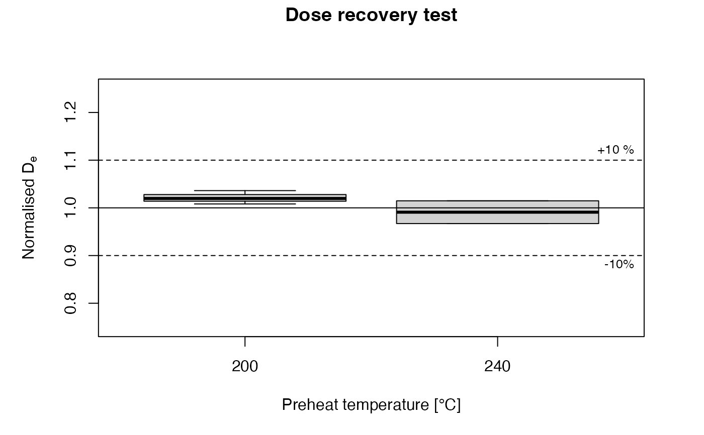
The function provides a standardised plot output for dose recovery test measurements.
Usage
plot_DRTResults(
  object,
  given.dose = NULL,
  error.range = 10,
  preheat = NULL,
  boxplot = FALSE,
  mtext = "",
  summary = "",
  summary.pos = "topleft",
  legend = NULL,
  legend.pos = "topright",
  par.local = TRUE,
  na.rm = FALSE,
  ...
)
Arguments
- object
RLum.Results or data.frame (required): input values containing at least De and De error. To plot more than one data set in one figure, a
listof the individual data sets must be provided (e.g.list(dataset.1, dataset.2)).- given.dose
numeric (optional): given dose used for the dose recovery test to normalise data. If only one given dose is provided, this given dose is valid for all input data sets (i.e.,
objectis a list). Otherwise, a given dose for each input data set has to be provided (e.g.,given.dose = c(100,200)). Ifgiven.doseisNULLor 0, the values are plotted without normalisation (might be useful for preheat plateau tests). Note: Unit has to be the same as from the input values (e.g., Seconds or Gray).- error.range
numeric (with default): symmetric error range in percent will be shown as dashed lines in the plot. It can be set to 0 to remove the error ranges.
- preheat
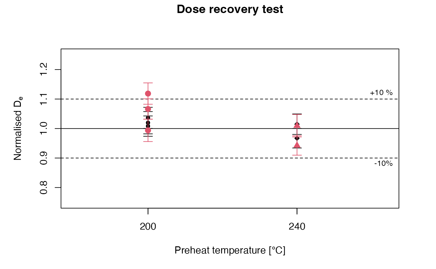
numeric (optional): optional vector of preheat temperatures to be used for grouping the De values. If specified, the temperatures are assigned to the x-axis.
- boxplot
logical (with default): plot values that are grouped by preheat temperature as boxplots. Only possible when
preheatvector is specified.- mtext
character (with default): additional text below the plot title.
- summary
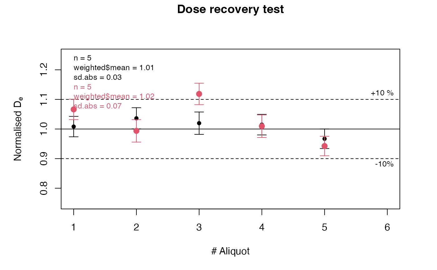
character (optional): adds numerical output to the plot. Can be one or more out of:
"n"(number of samples),"mean"(mean De value),"weighted$mean"(error-weighted mean),"median"(median of the De values),"weighted$median"(error-weighted median),"sd.rel"(relative standard deviation in percent),"sd.abs"(absolute standard deviation),"se.rel"(relative standard error) and"se.abs"(absolute standard error)
and all other measures returned by the function calc_Statistics.
- summary.pos
numeric or character (with default): optional position coordinates or keyword (e.g.
"topright") for the statistical summary. Alternatively, the keyword"sub"may be specified to place the summary below the plot header. However, this latter option in only possible ifmtextis not used.- legend
character vector (optional): legend content to be added to the plot.
- legend.pos
numeric or character (with default): optional position coordinates or keyword (e.g.
"topright") for the legend to be plotted.- par.local
logical (with default): use local graphical parameters for plotting, e.g. the plot is shown in one column and one row. If
par.local = FALSE, global parameters are inherited, i.e. parameters provided viapar()work.- na.rm
logical (with default): whether
NAvalues should be removed from the input data before plotting.- ...
further arguments and graphical parameters passed to plot, supported are:
xlab,ylab,xlim,ylim,main,cex,lasandpch.
Details
The procedure tests the accuracy of a measurement protocol to reliably
determine the dose of a specific sample. Here, the natural signal is erased
and a known laboratory dose administered, which is treated as unknown. Then
the De measurement is carried out and the degree of congruence between
administered and recovered dose is a measure of the protocol's accuracy for
this sample.
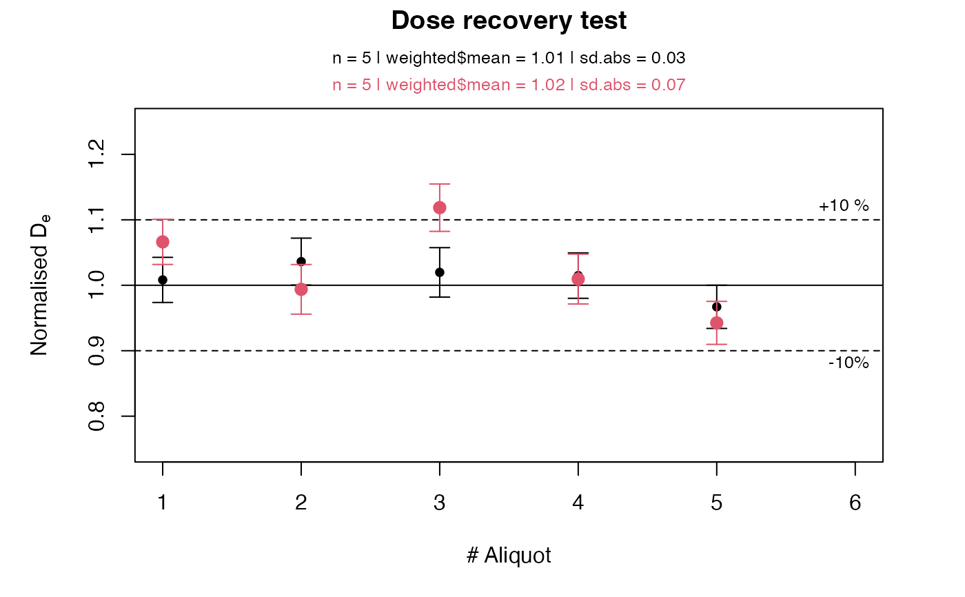
In the plot the normalised De is shown on the y-axis, i.e. obtained De/Given Dose.
How to cite
Kreutzer, S., Dietze, M., 2026. plot_DRTResults(): Visualise dose recovery test results. Function version 0.1.17. In: Kreutzer, S., Burow, C., Dietze, M., Fuchs, M.C., Schmidt, C., Fischer, M., Friedrich, J., Mercier, N., Philippe, A., Riedesel, S., Autzen, M., Mittelstrass, D., Gray, H.J., Galharret, J., Colombo, M., Steinbuch, L., Boer, A.d., Bluszcz, A., 2026. Luminescence: Comprehensive Luminescence Dating Data Analysis. R package version 1.2.1. https://r-lum.github.io/Luminescence/
References
Wintle, A.G., Murray, A.S., 2006. A review of quartz optically stimulated luminescence characteristics and their relevance in single-aliquot regeneration dating protocols. Radiation Measurements 41, 369-391.
Author
Sebastian Kreutzer, F2.1 Geophysical Parametrisation/Regionalisation, LIAG - Institute for Applied Geophysics (Germany)
Michael Dietze, GFZ Potsdam (Germany)
, RLum Developer Team
Examples
## read example data set and misapply them for this plot type
data(ExampleData.DeValues, envir = environment())
## plot values
plot_DRTResults(
ExampleData.DeValues$BT998[7:11,],
given.dose = 2800,
mtext = "Example data")
 ## plot values with legend
plot_DRTResults(
ExampleData.DeValues$BT998[7:11,],
given.dose = 2800,
legend = "Test data set")
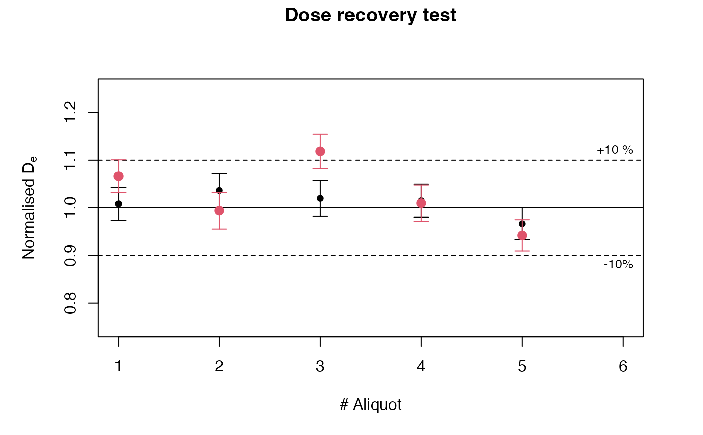
 ## create and plot two subsets with randomised values
x.1 <- ExampleData.DeValues$BT998[7:11,]
x.2 <- ExampleData.DeValues$BT998[7:11,] * c(runif(5, 0.9, 1.1), 1)
plot_DRTResults(
list(x.1, x.2),
given.dose = 2800)
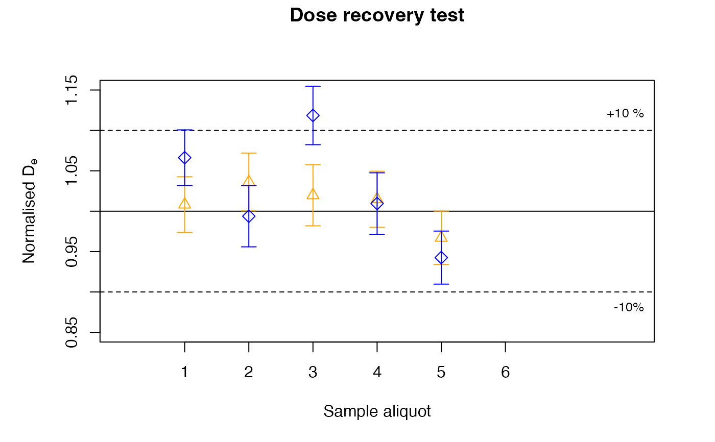
 ## some more user-defined plot parameters
plot_DRTResults(
list(x.1, x.2),
given.dose = 2800,
pch = c(2, 5),
col = c("orange", "blue"),
xlim = c(0, 8),
ylim = c(0.85, 1.15),
xlab = "Sample aliquot")
 ## plot the data with user-defined statistical measures as legend
plot_DRTResults(
list(x.1, x.2),
given.dose = 2800,
summary = c("n", "weighted$mean", "sd.abs"))
 ## plot the data with user-defined statistical measures as sub-header
plot_DRTResults(
list(x.1, x.2),
given.dose = 2800,
summary = c("n", "weighted$mean", "sd.abs"),
summary.pos = "sub")
 ## plot the data grouped by preheat temperatures
plot_DRTResults(
ExampleData.DeValues$BT998[7:11,],
given.dose = 2800,
preheat = c(200, 200, 200, 240, 240))
 ## read example data set and misapply them for this plot type
data(ExampleData.DeValues, envir = environment())
## plot values
plot_DRTResults(
ExampleData.DeValues$BT998[7:11,],
given.dose = 2800,
mtext = "Example data")
 ## plot two data sets grouped by preheat temperatures
plot_DRTResults(
list(x.1, x.2),
given.dose = 2800,
preheat = c(200, 200, 200, 240, 240))
 ## plot the data grouped by preheat temperatures as boxplots
plot_DRTResults(
ExampleData.DeValues$BT998[7:11,],
given.dose = 2800,
preheat = c(200, 200, 200, 240, 240),
boxplot = TRUE)
