Fit and plot a dose-response curve for luminescence data (Lx/Tx against dose)
Source:R/plot_GrowthCurve.R
plot_GrowthCurve.RdA dose-response curve is produced for luminescence measurements using a regenerative or additive protocol as implemented in fit_DoseResponseCurve and plot_DoseResponseCurve
Usage
plot_GrowthCurve(
  object,
  mode = "interpolation",
  fit.method = "EXP",
  output.plot = TRUE,
  output.plotExtended = TRUE,
  plot_singlePanels = FALSE,
  verbose = TRUE,
  n.MC = 100,
  ...
)
Arguments
- object
data.frame or a list of such objects (required): data frame with columns for
Dose,LxTx,LxTx.ErrorandTnTx. The column for the test dose response is optional, but requires'TnTx'as column name if used. For exponential fits at least three dose points (including the natural) should be provided. Ifobjectis a list, the function is called on each of its elements. Iffit.method = "OTORX"you have to provide the test dose in the same unit as the dose in a column calledTest_Dose. The function searches explicitly for this column name. Only the first value will be used assuming a constant test dose over the measurement cycle.- mode
character (with default): selects calculation mode of the function.
"interpolation"(default) calculates the De by interpolation,"extrapolation"calculates the equivalent dose by extrapolation (useful for MAAD measurements) and"alternate"calculates no equivalent dose and just fits the data points.
Please note that for option
"interpolation"the first point is considered as natural dose- fit.method
character (with default): function used for fitting. Possible options are:
LIN,QDR,EXP,EXP OR LIN,EXP+LIN,EXP+EXP(not defined for extrapolation),GOK,OTORandOTORX. See details.- output.plot
logical (with default): enable/disable the plot output.
- output.plotExtended
logical (with default): If
TRUE, 3 plots on one plot area are provided:growth curve,
histogram from Monte Carlo error simulation and
a test dose response plot.
If
FALSE, just the growth curve will be plotted.- plot_singlePanels
logical (with default): single plot output (
TRUE/FALSE) to allow for plotting the results in single plot windows. Requiresoutput.plotExtended = TRUE.- verbose
logical (with default): enable/disable output to the terminal.
- n.MC
integer (with default): number of MC runs for error calculation.
- ...
Further arguments to fit_DoseResponseCurve (
fit_weights,fit_bounds,fit.force_through_origin,fit.includingRepeatedRegPoints,fit.NumberRegPoints,fit.NumberRegPointsReal,n.MC,txtProgressBar) and graphical parameters to be passed (supported:xlim,ylim,main,xlab,ylab).
Value
Along with a plot (if wanted) the RLum.Results object produced by fit_DoseResponseCurve is returned.
How to cite
Kreutzer, S., Dietze, M., Colombo, M., 2026. plot_GrowthCurve(): Fit and plot a dose-response curve for luminescence data (Lx/Tx against dose). Function version 1.2.3. In: Kreutzer, S., Burow, C., Dietze, M., Fuchs, M.C., Schmidt, C., Fischer, M., Friedrich, J., Mercier, N., Philippe, A., Riedesel, S., Autzen, M., Mittelstrass, D., Gray, H.J., Galharret, J., Colombo, M., Steinbuch, L., Boer, A.d., Bluszcz, A., 2026. Luminescence: Comprehensive Luminescence Dating Data Analysis. R package version 1.2.1. https://r-lum.github.io/Luminescence/
References
Berger, G.W., Huntley, D.J., 1989. Test data for exponential fits. Ancient TL 7, 43-46.
Guralnik, B., Li, B., Jain, M., Chen, R., Paris, R.B., Murray, A.S., Li, S.-H., Pagonis, P., Herman, F., 2015. Radiation-induced growth and isothermal decay of infrared-stimulated luminescence from feldspar. Radiation Measurements 81, 224-231.
Pagonis, V., Kitis, G., Chen, R., 2020. A new analytical equation for the dose response of dosimetric materials, based on the Lambert W function. Journal of Luminescence 225, 117333. doi:10.1016/j.jlumin.2020.117333
Author
Sebastian Kreutzer, F2.1 Geophysical Parametrisation/Regionalisation, LIAG - Institute for Applied Geophysics (Germany)
Michael Dietze, GFZ Potsdam (Germany)
Marco Colombo, Institute of Geography, Heidelberg University (Germany)
, RLum Developer Team
Examples
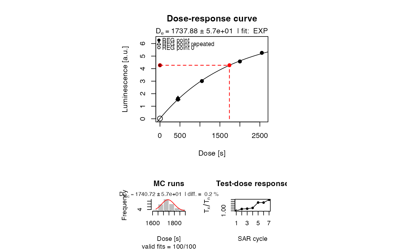
##(1) plot growth curve for a dummy dataset
data(ExampleData.LxTxData, envir = environment())
plot_GrowthCurve(LxTxData)
#> [fit_DoseResponseCurve()] Fit: EXP (interpolation) | De = 1737.88 | D01 = 1766.07
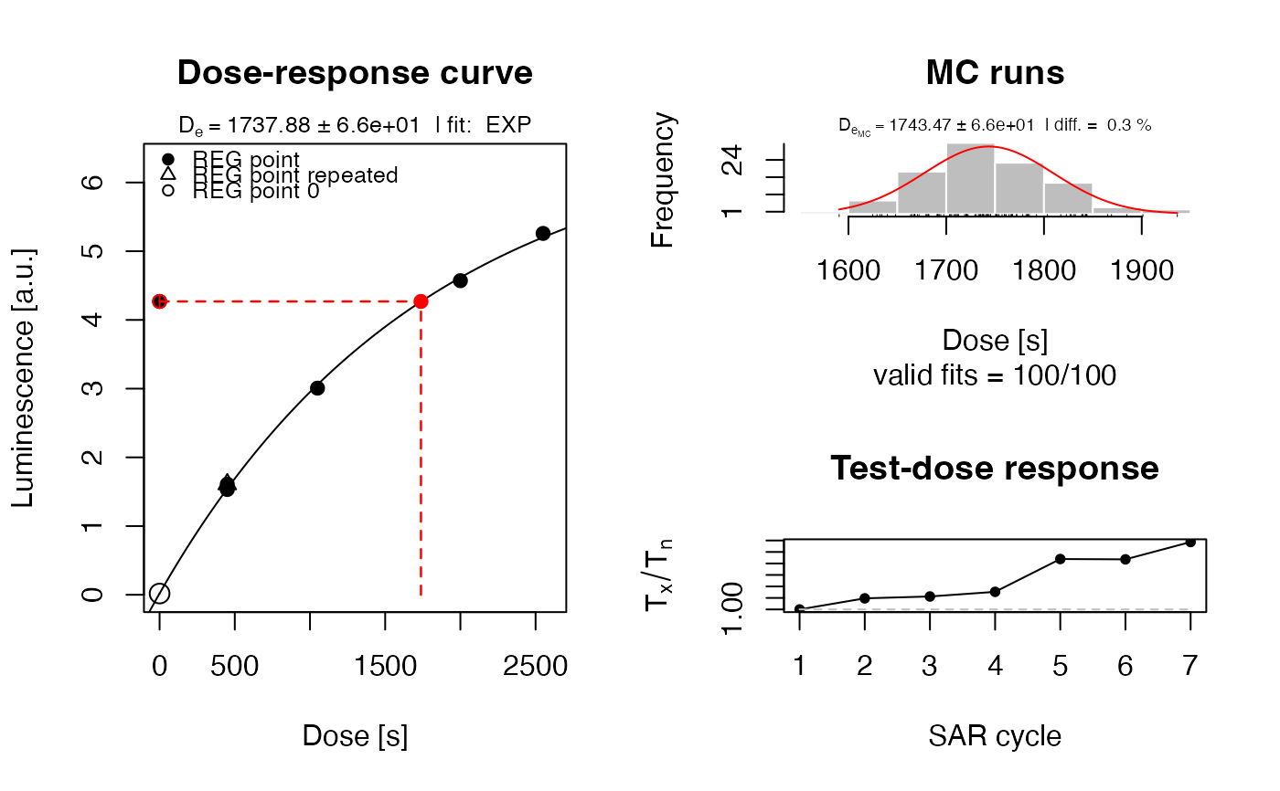
 ##(1b) horizontal plot arrangement
layout(mat = matrix(c(1,1,2,3), ncol = 2))
plot_GrowthCurve(LxTxData, plot_singlePanels = TRUE)
#> [fit_DoseResponseCurve()] Fit: EXP (interpolation) | De = 1737.88 | D01 = 1766.07
##(1b) horizontal plot arrangement
layout(mat = matrix(c(1,1,2,3), ncol = 2))
plot_GrowthCurve(LxTxData, plot_singlePanels = TRUE)
#> [fit_DoseResponseCurve()] Fit: EXP (interpolation) | De = 1737.88 | D01 = 1766.07
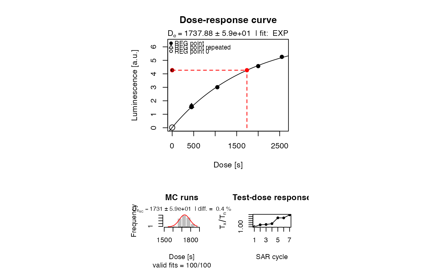
 ##(2) plot the growth curve with pdf output - uncomment to use
##pdf(file = "~/Desktop/Growth_Curve_Dummy.pdf", paper = "special")
plot_GrowthCurve(LxTxData)
#> [fit_DoseResponseCurve()] Fit: EXP (interpolation) | De = 1737.88 | D01 = 1766.07
##(2) plot the growth curve with pdf output - uncomment to use
##pdf(file = "~/Desktop/Growth_Curve_Dummy.pdf", paper = "special")
plot_GrowthCurve(LxTxData)
#> [fit_DoseResponseCurve()] Fit: EXP (interpolation) | De = 1737.88 | D01 = 1766.07
 ##dev.off()
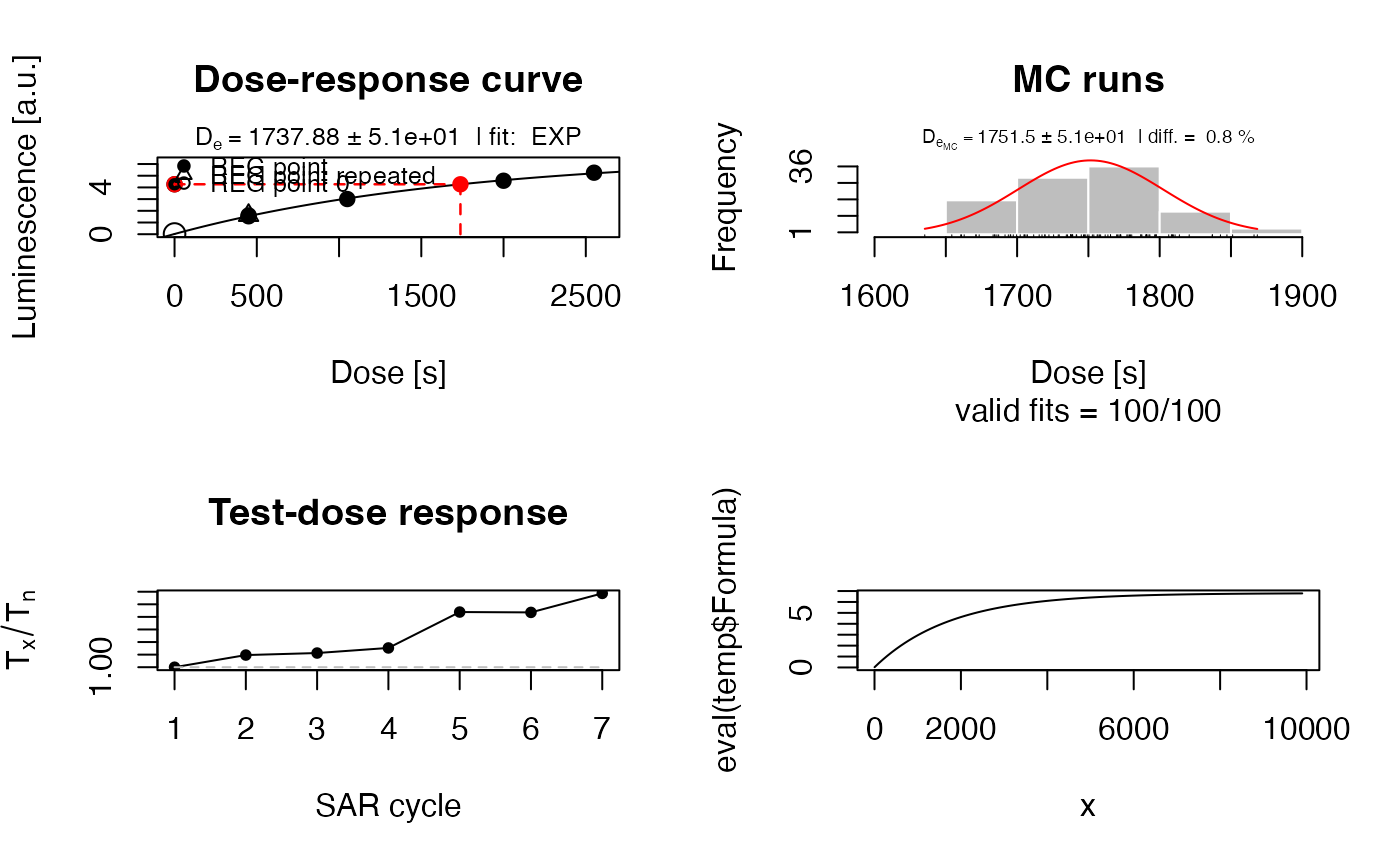
##(3) plot the growth curve with pdf output - uncomment to use, single output
##pdf(file = "~/Desktop/Growth_Curve_Dummy.pdf", paper = "special")
temp <- plot_GrowthCurve(LxTxData, plot_singlePanels = TRUE)
#> [fit_DoseResponseCurve()] Fit: EXP (interpolation) | De = 1737.88 | D01 = 1766.07
##dev.off()
##(4) plot resulting function for given interval x
x <- seq(1,10000, by = 100)
plot(
x = x,
y = eval(temp$Formula),
type = "l"
)
##dev.off()
##(3) plot the growth curve with pdf output - uncomment to use, single output
##pdf(file = "~/Desktop/Growth_Curve_Dummy.pdf", paper = "special")
temp <- plot_GrowthCurve(LxTxData, plot_singlePanels = TRUE)
#> [fit_DoseResponseCurve()] Fit: EXP (interpolation) | De = 1737.88 | D01 = 1766.07
##dev.off()
##(4) plot resulting function for given interval x
x <- seq(1,10000, by = 100)
plot(
x = x,
y = eval(temp$Formula),
type = "l"
)
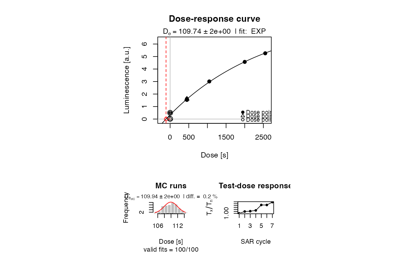
 ##(5) plot using the 'extrapolation' mode
LxTxData[1,2:3] <- c(0.5, 0.001)
print(plot_GrowthCurve(LxTxData, mode = "extrapolation"))
#> [fit_DoseResponseCurve()] Fit: EXP (extrapolation) | De = 109.74 | D01 = 2624.06
##(5) plot using the 'extrapolation' mode
LxTxData[1,2:3] <- c(0.5, 0.001)
print(plot_GrowthCurve(LxTxData, mode = "extrapolation"))
#> [fit_DoseResponseCurve()] Fit: EXP (extrapolation) | De = 109.74 | D01 = 2624.06
 #>
#> [RLum.Results-class]
#> originator: fit_DoseResponseCurve()
#> data: 5
#> .. $De : data.frame
#> .. $De.MC : numeric
#> .. $Fit : nls
#> .. $Fit.Args : list
#> .. $Formula : expression
#> additional info elements: 2
##(6) plot using the 'alternate' mode
LxTxData[1,2:3] <- c(0.5, 0.001)
print(plot_GrowthCurve(LxTxData, mode = "alternate"))
#> [fit_DoseResponseCurve()] Fit: EXP (alternate) | De = NA | D01 = 2624.06
#>
#> [RLum.Results-class]
#> originator: fit_DoseResponseCurve()
#> data: 5
#> .. $De : data.frame
#> .. $De.MC : numeric
#> .. $Fit : nls
#> .. $Fit.Args : list
#> .. $Formula : expression
#> additional info elements: 2
##(6) plot using the 'alternate' mode
LxTxData[1,2:3] <- c(0.5, 0.001)
print(plot_GrowthCurve(LxTxData, mode = "alternate"))
#> [fit_DoseResponseCurve()] Fit: EXP (alternate) | De = NA | D01 = 2624.06
 #>
#> [RLum.Results-class]
#> originator: fit_DoseResponseCurve()
#> data: 5
#> .. $De : data.frame
#> .. $De.MC : numeric
#> .. $Fit : nls
#> .. $Fit.Args : list
#> .. $Formula : expression
#> additional info elements: 2
#>
#> [RLum.Results-class]
#> originator: fit_DoseResponseCurve()
#> data: 5
#> .. $De : data.frame
#> .. $De.MC : numeric
#> .. $Fit : nls
#> .. $Fit.Args : list
#> .. $Formula : expression
#> additional info elements: 2