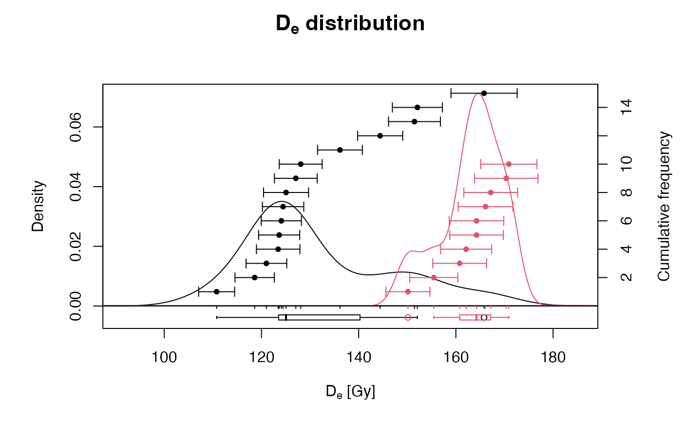
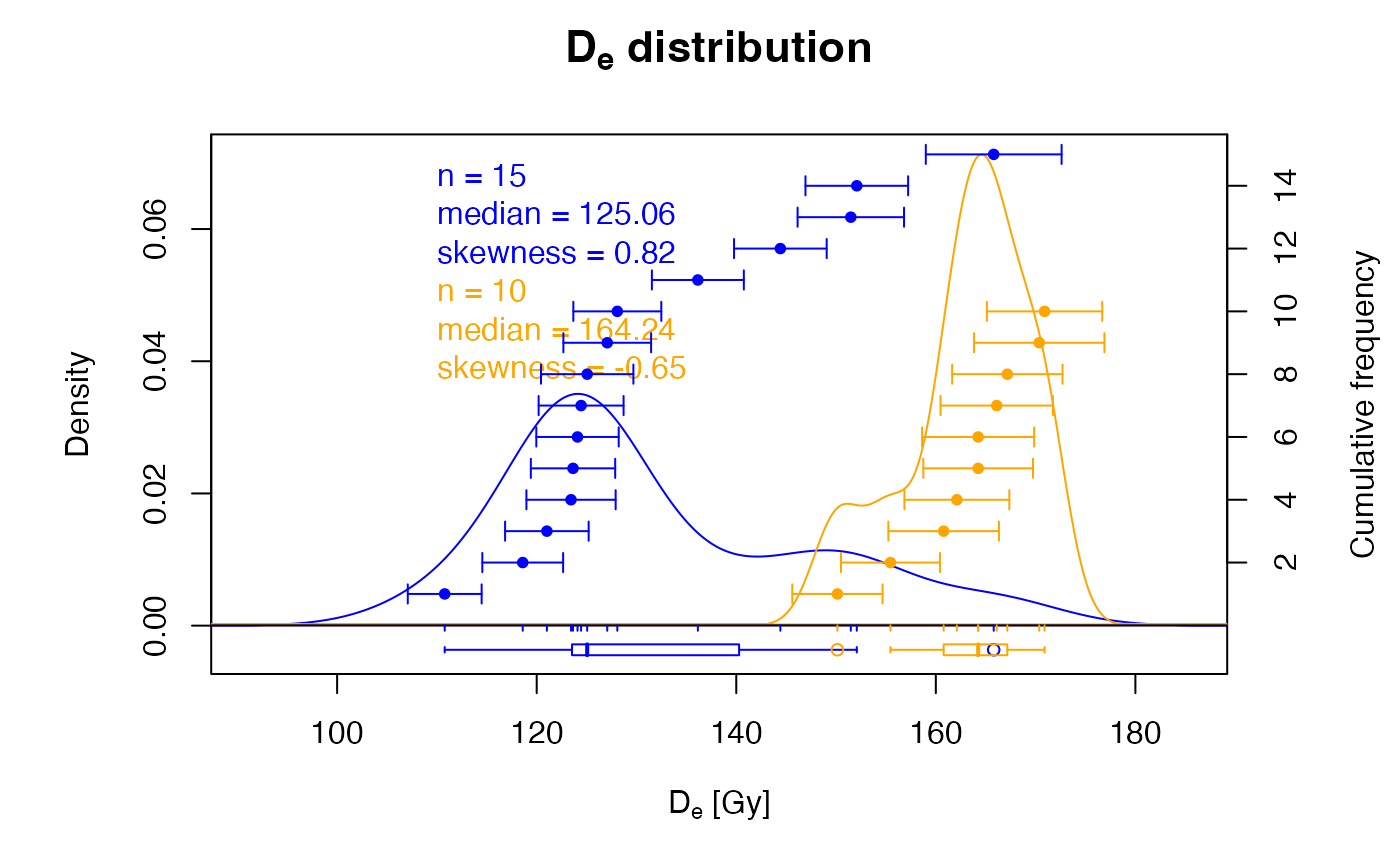
Plot kernel density estimate with statistics

Plot a kernel density estimate of measurement values in combination with the actual values and associated error bars in ascending order. If enabled, the boxplot will show the usual distribution parameters (median as bold line, box delimited by the first and third quartile, whiskers defined by the extremes and outliers shown as points) and also the mean and standard deviation as pale bold line and pale polygon, respectively.

Usage

plot_KDE(
  data,
  na.rm = TRUE,
  values.cumulative = TRUE,
  order = TRUE,
  boxplot = TRUE,
  rug = TRUE,
  summary,
  summary.pos,
  summary.method = "MCM",
  bw = "nrd0",
  output = TRUE,
  ...
)

Arguments

data: data.frame, vector or RLum.Results object (required): for data.frame: either two columns: De (values[,1]) and De error (values[,2]), or one: De (values[,1]). If a numeric vector or a single-column data frame is provided, De error is assumed to be 10^-9 for all measurements and error bars are not drawn. For plotting multiple data sets, these must be provided as list (e.g. list(dataset1, dataset2)).
na.rm: logical (with default): exclude NA values from the data set prior to any further operation.
values.cumulative: logical (with default): show cumulative individual data.
order: logical: Order data in ascending order.
boxplot: logical (with default): optionally show a boxplot (depicting median as thick central line, first and third quartile as box limits, whiskers denoting +/- 1.5 interquartile ranges and dots further outliers).
rug: logical (with default): optionally add rug.
summary: character (optional): add statistic measures of centrality and dispersion to the plot. Can be one or more of several keywords. See details for available keywords.
summary.pos: numeric or character (with default): optional position coordinates or keyword (e.g. "topright") for the statistical summary. Alternatively, the keyword "sub" may be specified to place the summary below the plot header. However, this latter option in only possible if mtext is not used. In case of coordinate specification, y-coordinate refers to the right y-axis.
summary.method: character (with default): keyword indicating the method used to calculate the statistic summary. One out of "unweighted", "weighted" and "MCM". See calc_Statistics for details.
bw: character (with default): bin-width, chose a numeric value for manual setting.
output: logical: Optional output of numerical plot parameters. These can be useful to reproduce similar plots. Default is TRUE.
...: further arguments and graphical parameters passed to plot.

Details

The function allows passing several plot arguments, such as main, xlab, cex. However, as the figure is an overlay of two separate plots, ylim must be specified in the order: c(ymin_axis1, ymax_axis1, ymin_axis2, ymax_axis2) when using the cumulative values plot option. See examples for some further explanations. For details on the calculation of the bin-width (parameter bw) see density.

A statistic summary, i.e. a collection of statistic measures of centrality and dispersion (and further measures) can be added by specifying one or more of the following keywords:

"n" (number of samples)
"mean" (mean De value)
"median" (median of the De values)
"sd.rel" (relative standard deviation in percent)
"sd.abs" (absolute standard deviation)
"se.rel" (relative standard error)
"se.abs" (absolute standard error)
"in.2s" (percent of samples in 2-sigma range)
"kurtosis" (kurtosis)
"skewness" (skewness)

Note that the input data for the statistic summary is sent to the function calc_Statistics() depending on the log-option for the z-scale. If "log.z = TRUE", the summary is based on the logarithms of the input data. If "log.z = FALSE" the linearly scaled data is used.

Note as well, that "calc_Statistics()" calculates these statistic measures in three different ways: unweighted, weighted and MCM-based (i.e., based on Monte Carlo Methods). By default, the MCM-based version is used. If you wish to use another method, indicate this with the appropriate keyword using the argument summary.method.

Note

The plot output is no 'probability density' plot (cf. the discussion of Berger and Galbraith in Ancient TL; see references)!

Function version

3.6.0

Author

Michael Dietze, GFZ Potsdam (Germany)
Geography & Earth Sciences, Aberystwyth University (United Kingdom) , RLum Developer Team

How to cite

Dietze, M., 2024. plot_KDE(): Plot kernel density estimate with statistics. Function version 3.6.0. In: Kreutzer, S., Burow, C., Dietze, M., Fuchs, M.C., Schmidt, C., Fischer, M., Friedrich, J., Mercier, N., Philippe, A., Riedesel, S., Autzen, M., Mittelstrass, D., Gray, H.J., Galharret, J., Colombo, M., 2024. Luminescence: Comprehensive Luminescence Dating Data Analysis. R package version 0.9.26. https://r-lum.github.io/Luminescence/

Examples


## read example data set
data(ExampleData.DeValues, envir = environment())
ExampleData.DeValues <-
  Second2Gray(ExampleData.DeValues$BT998, c(0.0438,0.0019))

## create plot straightforward
plot_KDE(data = ExampleData.DeValues)


## create plot with logarithmic x-axis
plot_KDE(data = ExampleData.DeValues,
         log = "x")


## create plot with user-defined labels and axes limits
plot_KDE(data = ExampleData.DeValues,
         main = "Dose distribution",
         xlab = "Dose (s)",
         ylab = c("KDE estimate", "Cumulative dose value"),
         xlim = c(100, 250),
         ylim = c(0, 0.08, 0, 30))


## create plot with boxplot option
plot_KDE(data = ExampleData.DeValues,
         boxplot = TRUE)


## create plot with statistical summary below header
plot_KDE(data = ExampleData.DeValues,
         summary = c("n", "median", "skewness", "in.2s"))


## create plot with statistical summary as legend
plot_KDE(data = ExampleData.DeValues,
         summary = c("n", "mean", "sd.rel", "se.abs"),
         summary.pos = "topleft")


## split data set into sub-groups, one is manipulated, and merge again
data.1 <- ExampleData.DeValues[1:15,]
data.2 <- ExampleData.DeValues[16:25,] * 1.3
data.3 <- list(data.1, data.2)

## create plot with two subsets straightforward
plot_KDE(data = data.3)


## create plot with two subsets and summary legend at user coordinates
plot_KDE(data = data.3,
         summary = c("n", "median", "skewness"),
         summary.pos = c(110, 0.07),
         col = c("blue", "orange"))


## example of how to use the numerical output of the function
## return plot output to draw a thicker KDE line
KDE_out <- plot_KDE(data = ExampleData.DeValues,
output = TRUE)