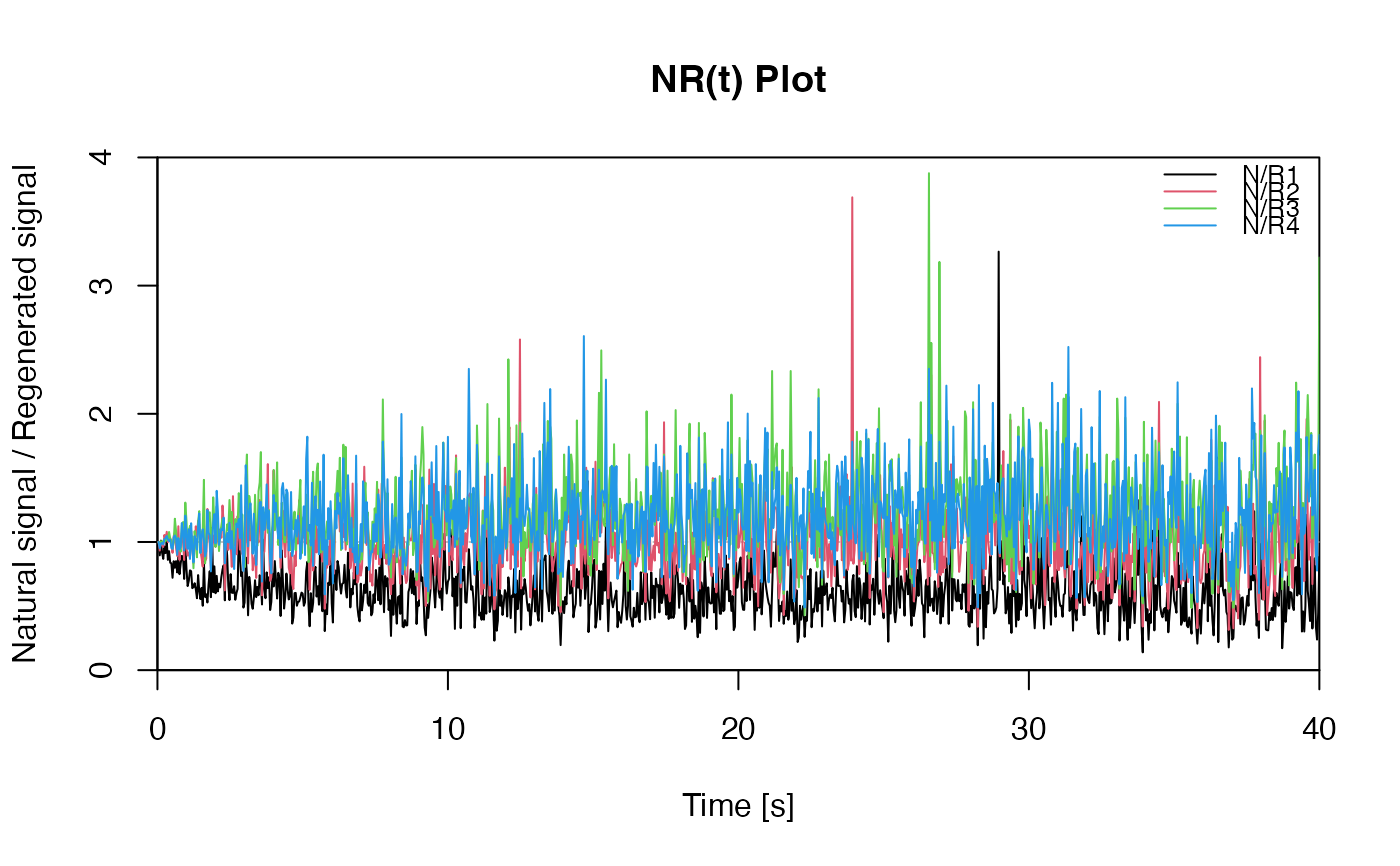
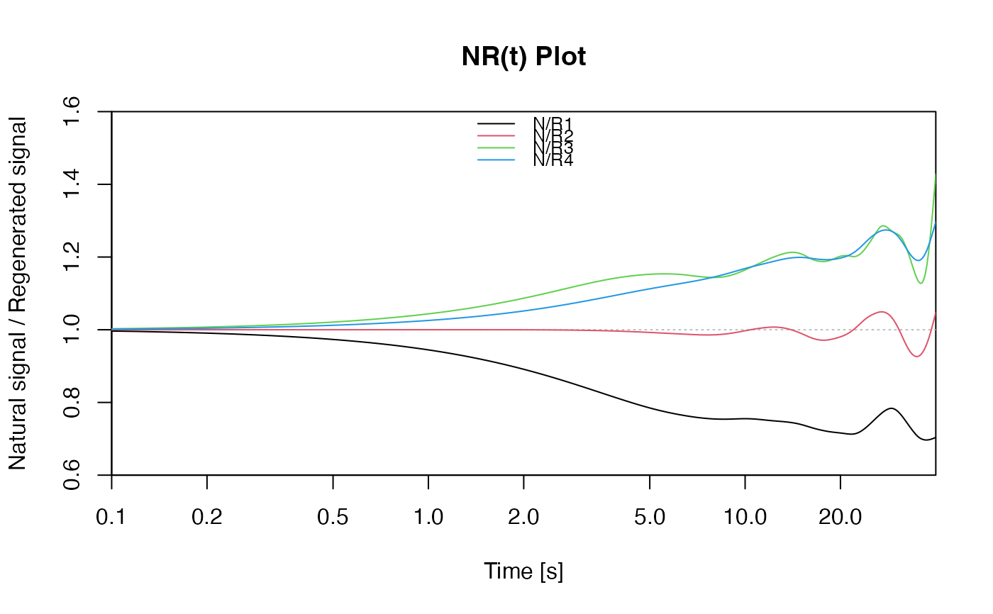
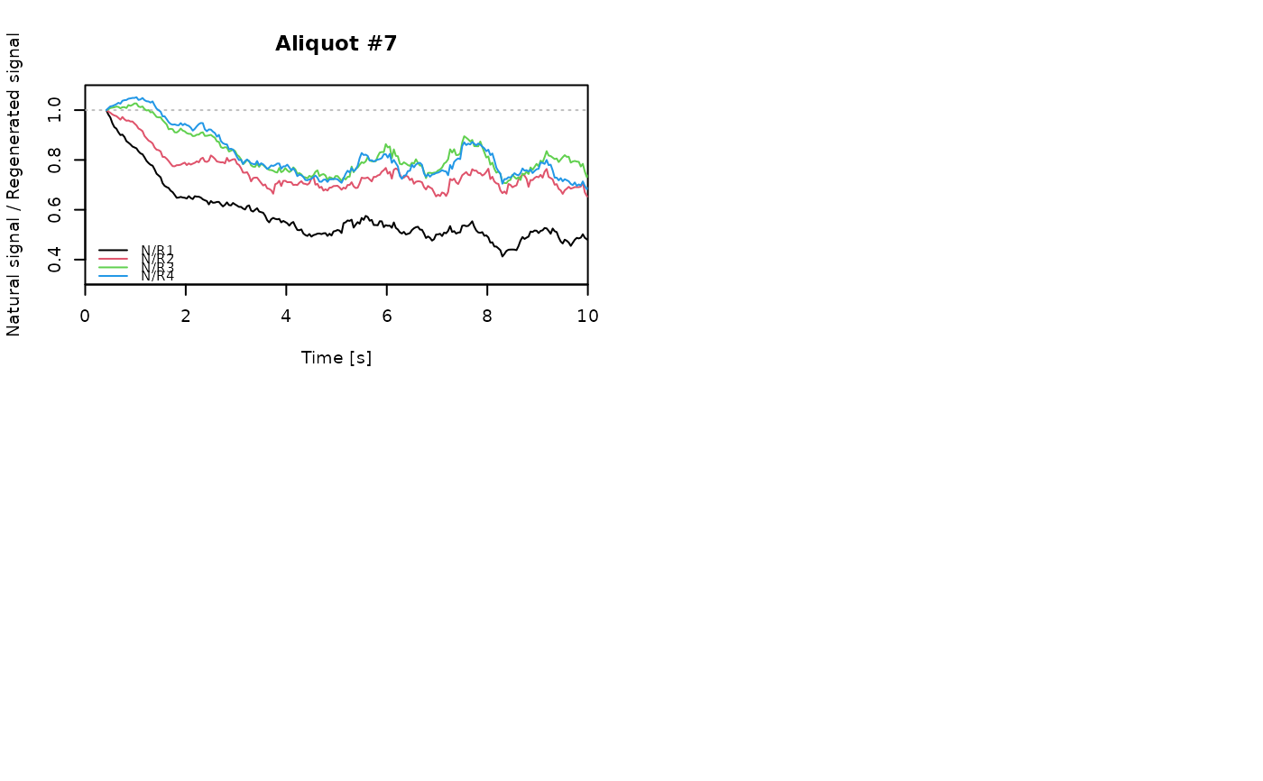
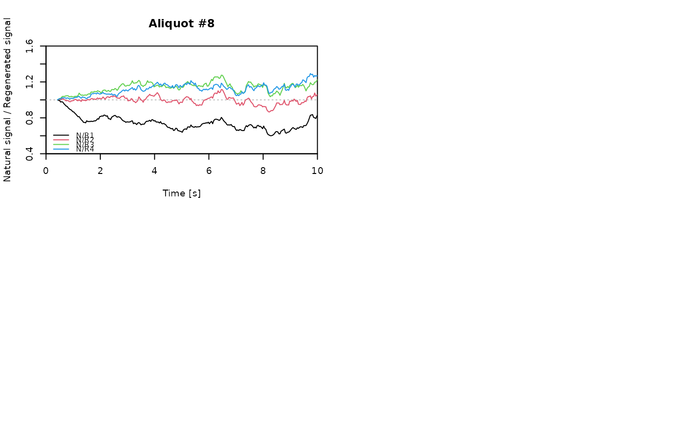
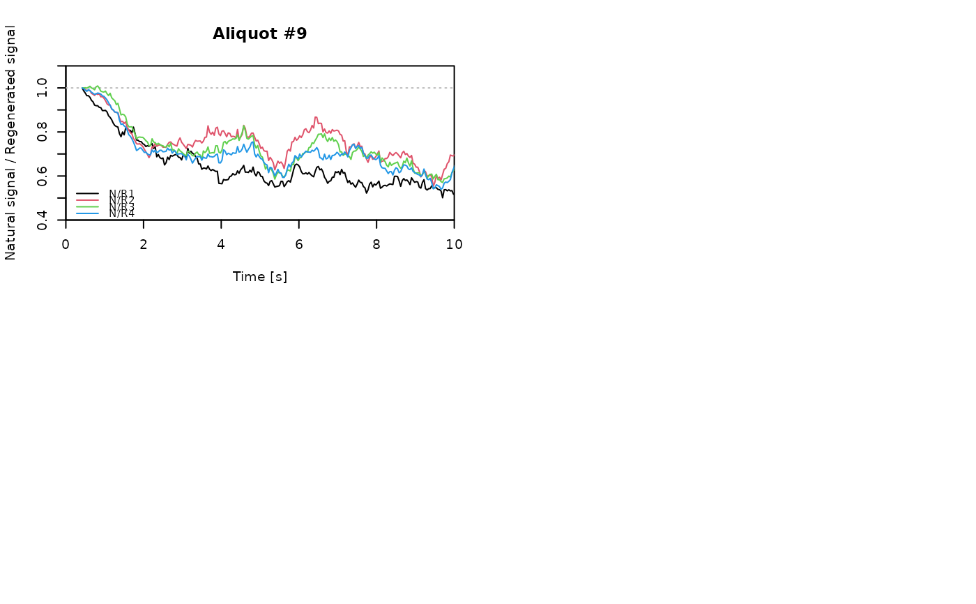
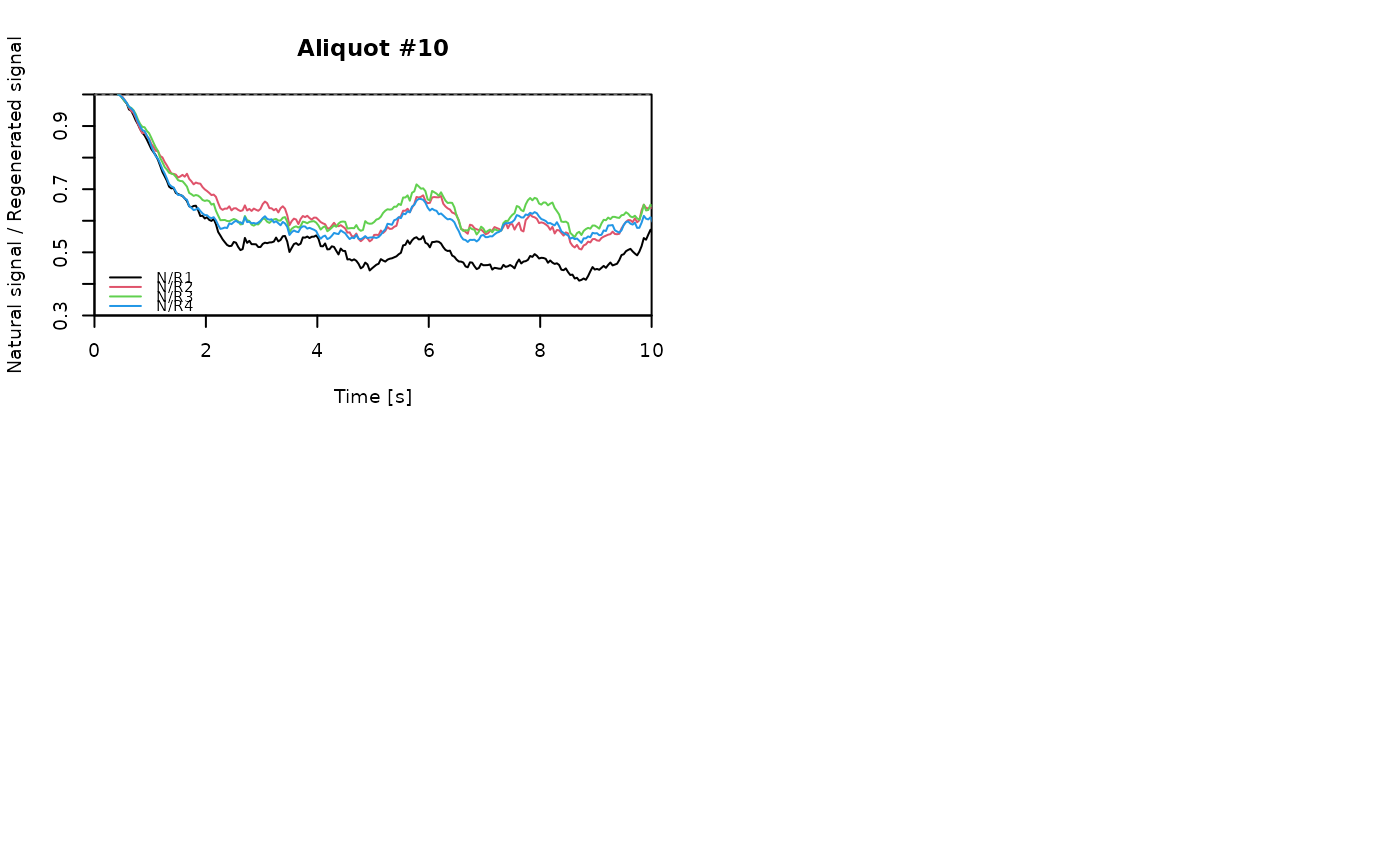
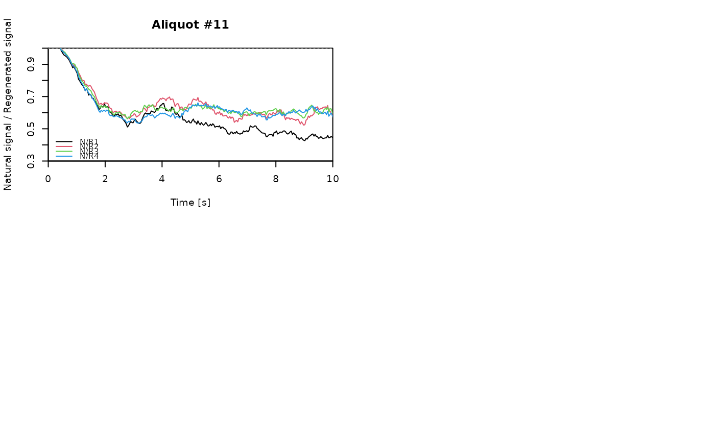
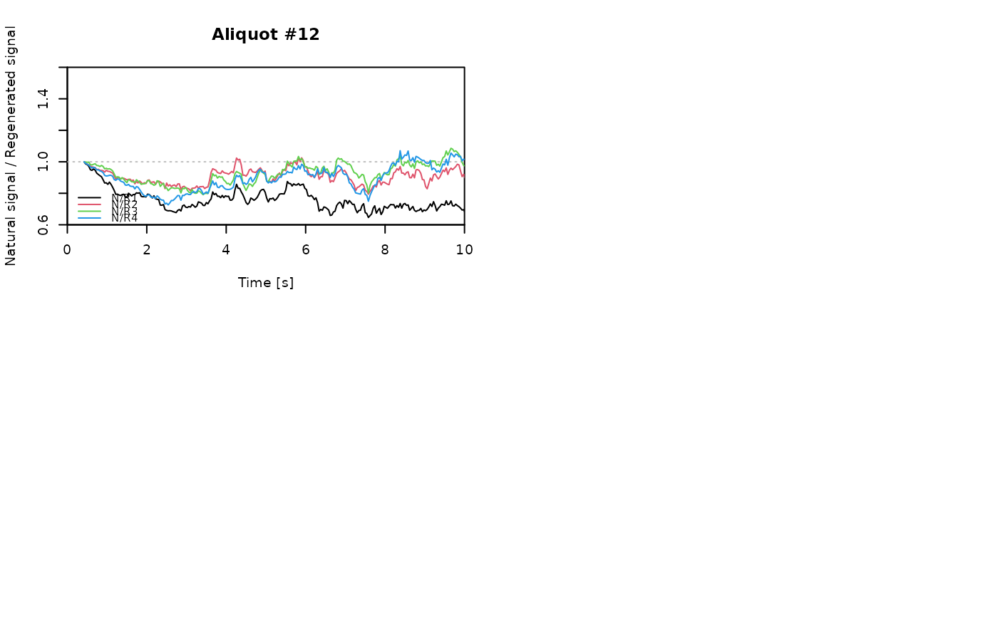
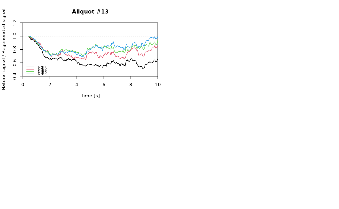
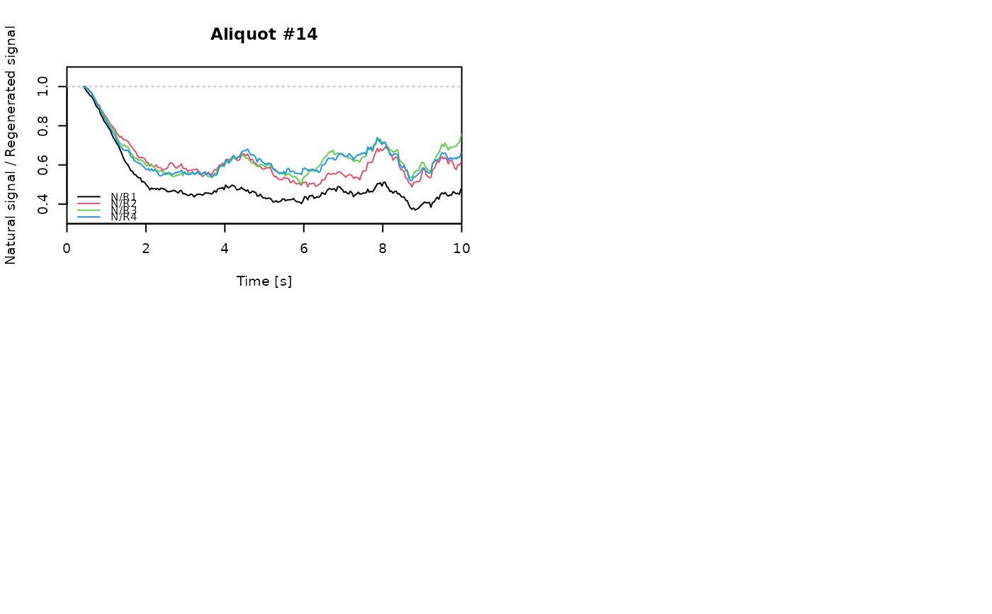
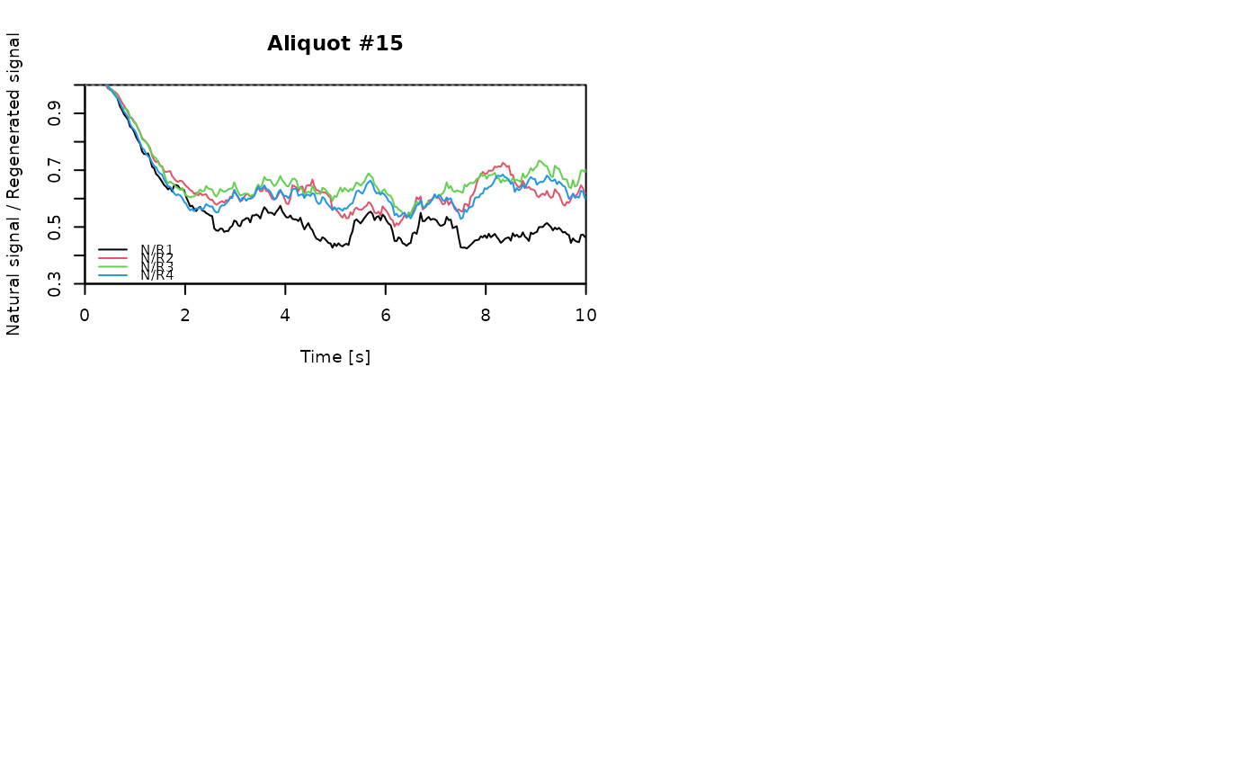
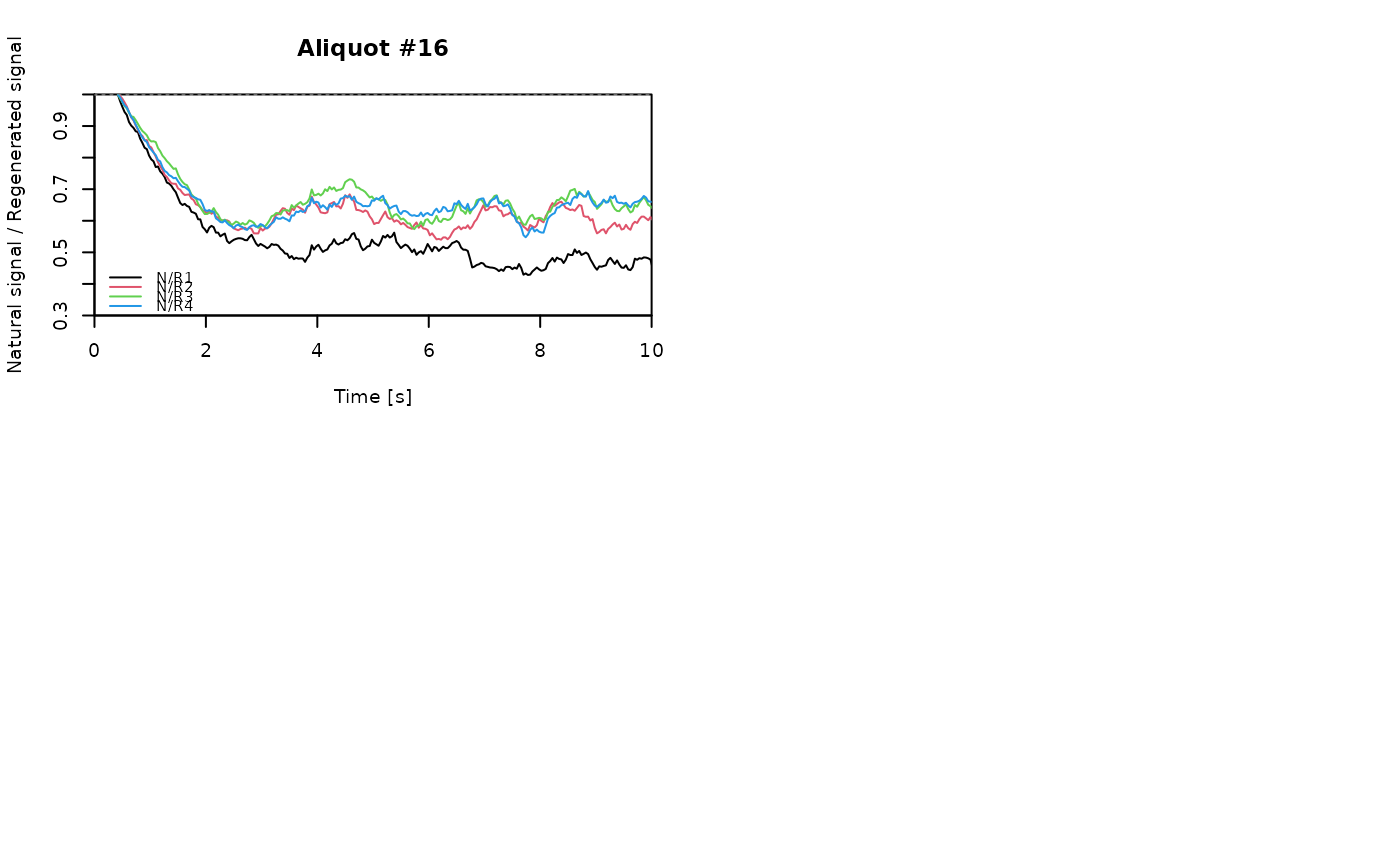
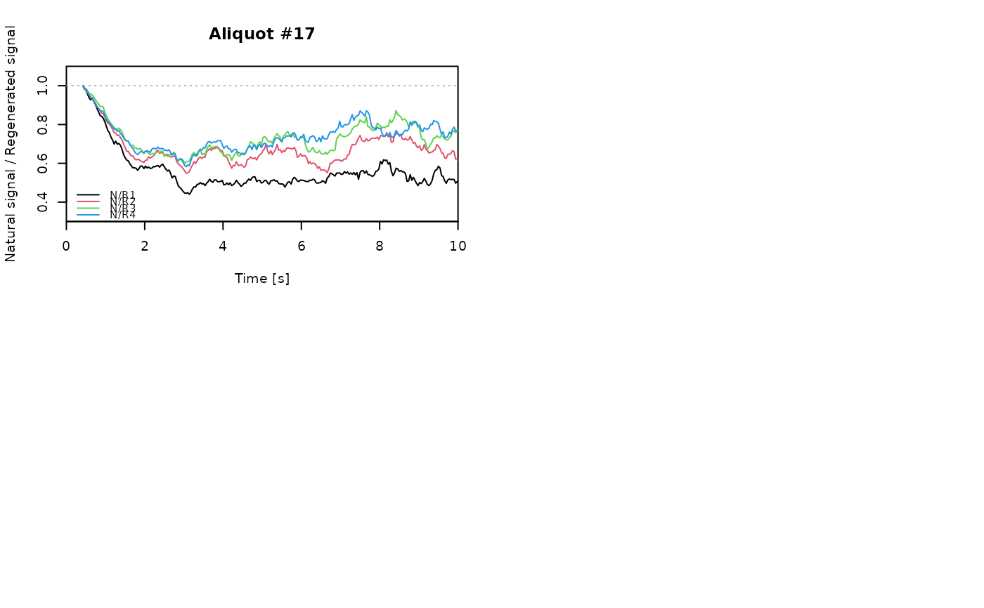
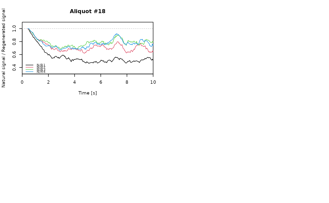
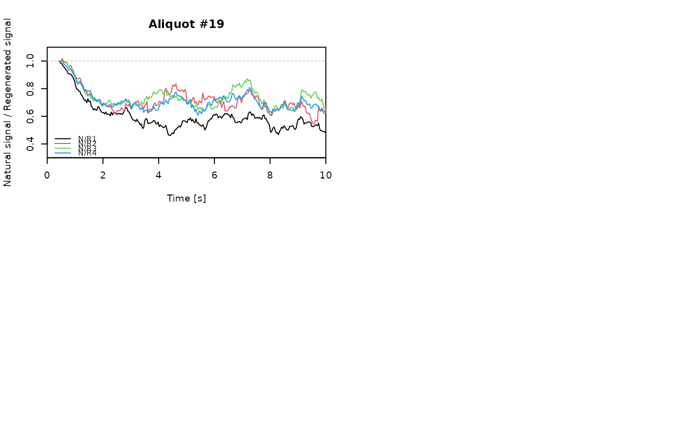
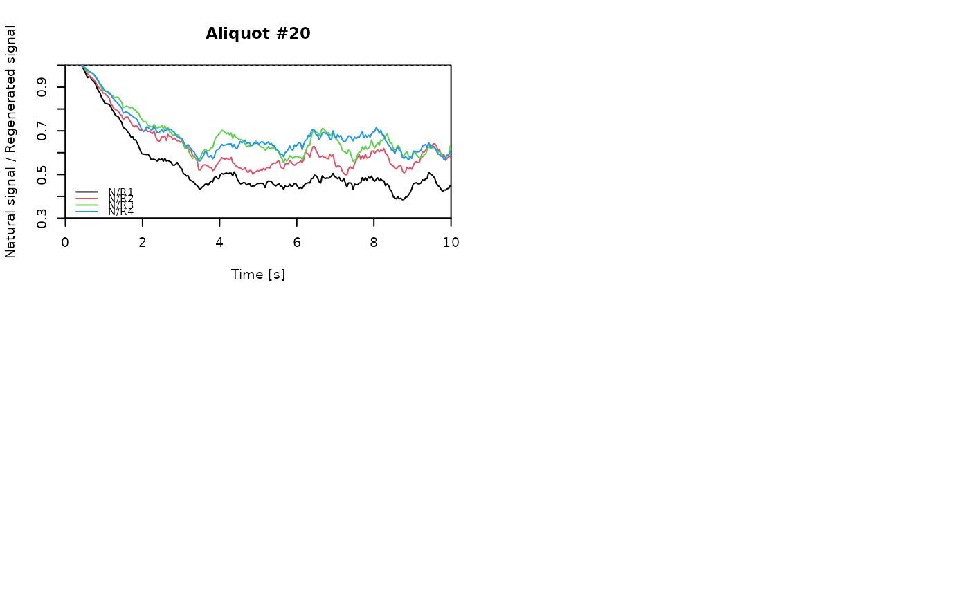
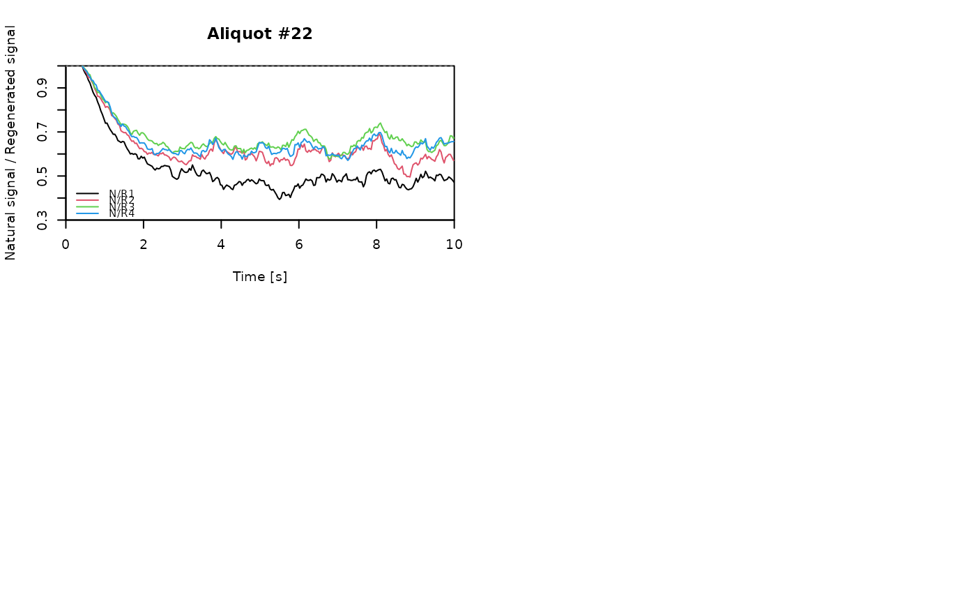
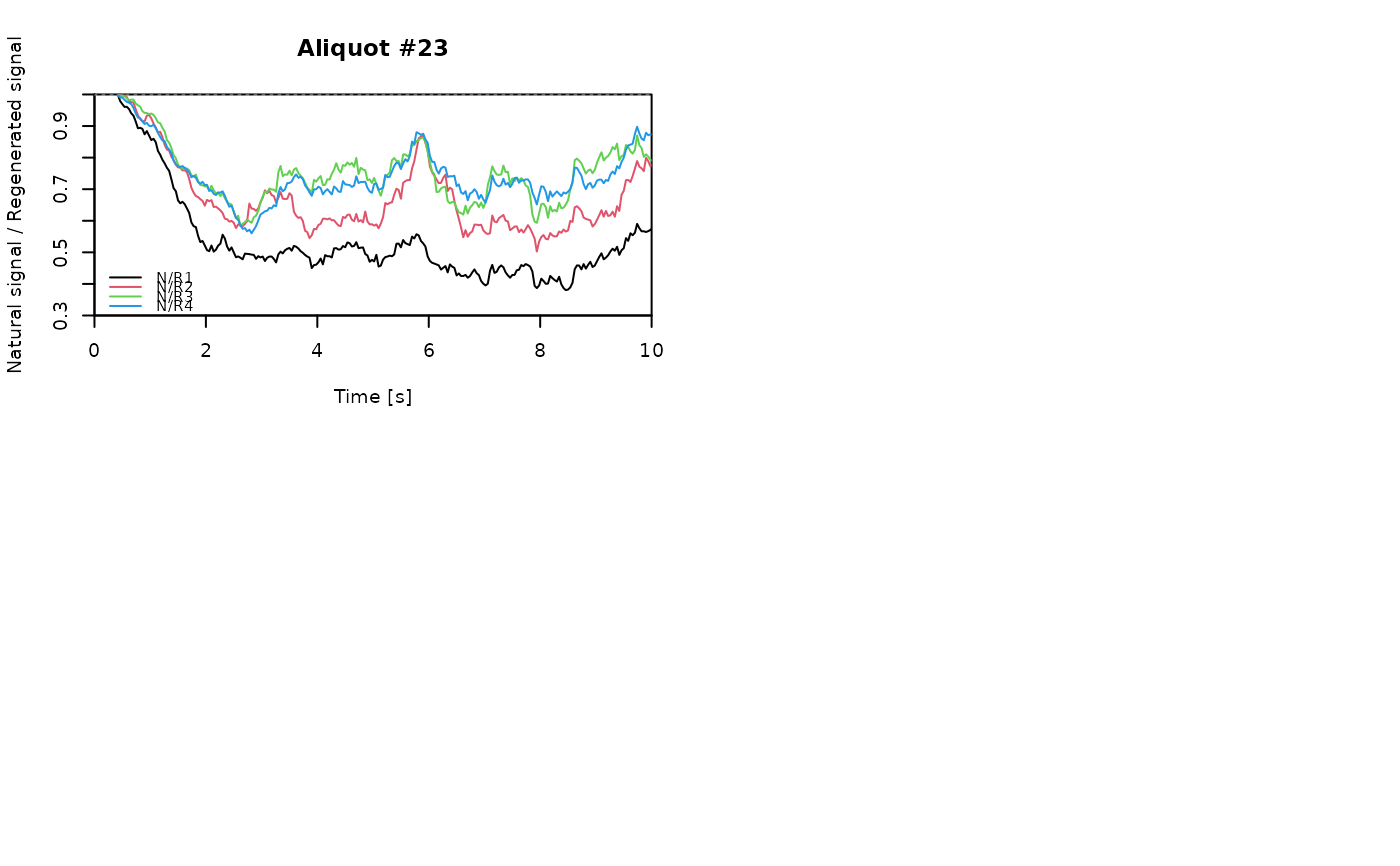
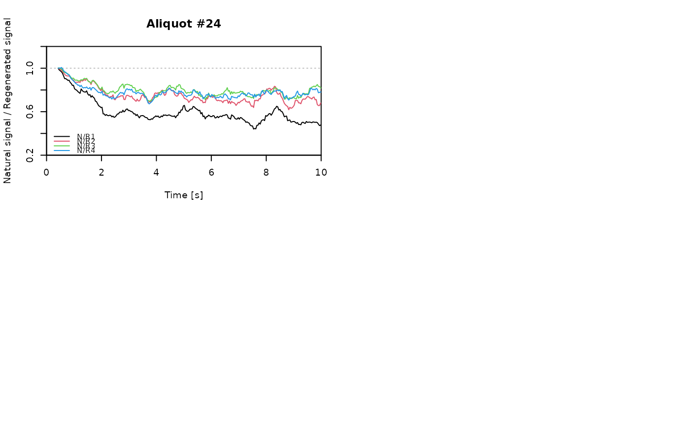
This function creates a Natural/Regenerated signal vs. time (NR(t)) plot as shown in Steffen et al. 2009.
This function accepts the individual curve data in many different formats. If
data is a list, each element of the list must contain a two
column data.frame or matrix containing the XY data of the curves
(time and counts). Alternatively, the elements can be objects of class
RLum.Data.Curve.
Input values can also be provided as a data.frame or matrix where
the first column contains the time values and each following column contains
the counts of each curve.
Usage
plot_NRt(
  data,
  log = "",
  smooth = c("none", "spline", "rmean"),
  k = 3,
  legend = TRUE,
  legend.pos = "topright",
  ...
)
Arguments
- data
list, data.frame, matrix or RLum.Analysis (required): X,Y data of measured values (time and counts). See details on individual data structure.
- log
character (with default): logarithmic axes (
"x","y","xy") or""(default) for linear axes.- smooth
character (with default): apply data smoothing. If
"none"(default), no data smoothing is applied. Use"rmean"to calculate the rolling mean, wherekdetermines the width of the rolling window (see data.table::frollmean)."spline"applies a smoothing spline to each curve (see stats::smooth.spline)- k
integer (with default): integer width of the rolling window.
- legend
logical (with default): enable/disable the plot legend.
- legend.pos
character (with default): keyword specifying the position of the legend (see legend).
- ...
Value
Returns a plot and RLum.Analysis object.
How to cite
Burow, C., 2026. plot_NRt(): Visualise natural/regenerated signal ratios. In: Kreutzer, S., Burow, C., Dietze, M., Fuchs, M.C., Schmidt, C., Fischer, M., Friedrich, J., Mercier, N., Philippe, A., Riedesel, S., Autzen, M., Mittelstrass, D., Gray, H.J., Galharret, J., Colombo, M., Steinbuch, L., Boer, A.d., Bluszcz, A., 2026. Luminescence: Comprehensive Luminescence Dating Data Analysis. R package version 1.2.1. https://r-lum.github.io/Luminescence/
References
Steffen, D., Preusser, F., Schlunegger, F., 2009. OSL quartz underestimation due to unstable signal components. Quaternary Geochronology, 4, 353-362.
Examples
## load example data
data("ExampleData.BINfileData", envir = environment())
## EXAMPLE 1
## convert Risoe.BINfileData object to RLum.Analysis object
data <- Risoe.BINfileData2RLum.Analysis(object = CWOSL.SAR.Data, pos = 8, ltype = "OSL")
## extract all OSL curves
allCurves <- get_RLum(data)
## keep only the natural and regenerated signal curves
pos <- seq(1, 9, 2)
curves <- allCurves[pos]
## plot a standard NR(t) plot
plot_NRt(curves)
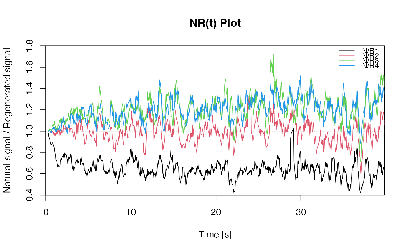
 ## re-plot with rolling mean data smoothing
plot_NRt(curves, smooth = "rmean", k = 10)
## re-plot with rolling mean data smoothing
plot_NRt(curves, smooth = "rmean", k = 10)
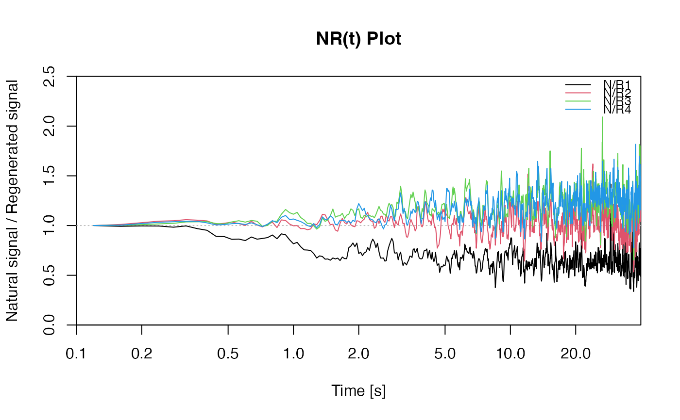
 ## re-plot with a logarithmic x-axis
plot_NRt(curves, log = "x", smooth = "rmean", k = 5)
## re-plot with a logarithmic x-axis
plot_NRt(curves, log = "x", smooth = "rmean", k = 5)
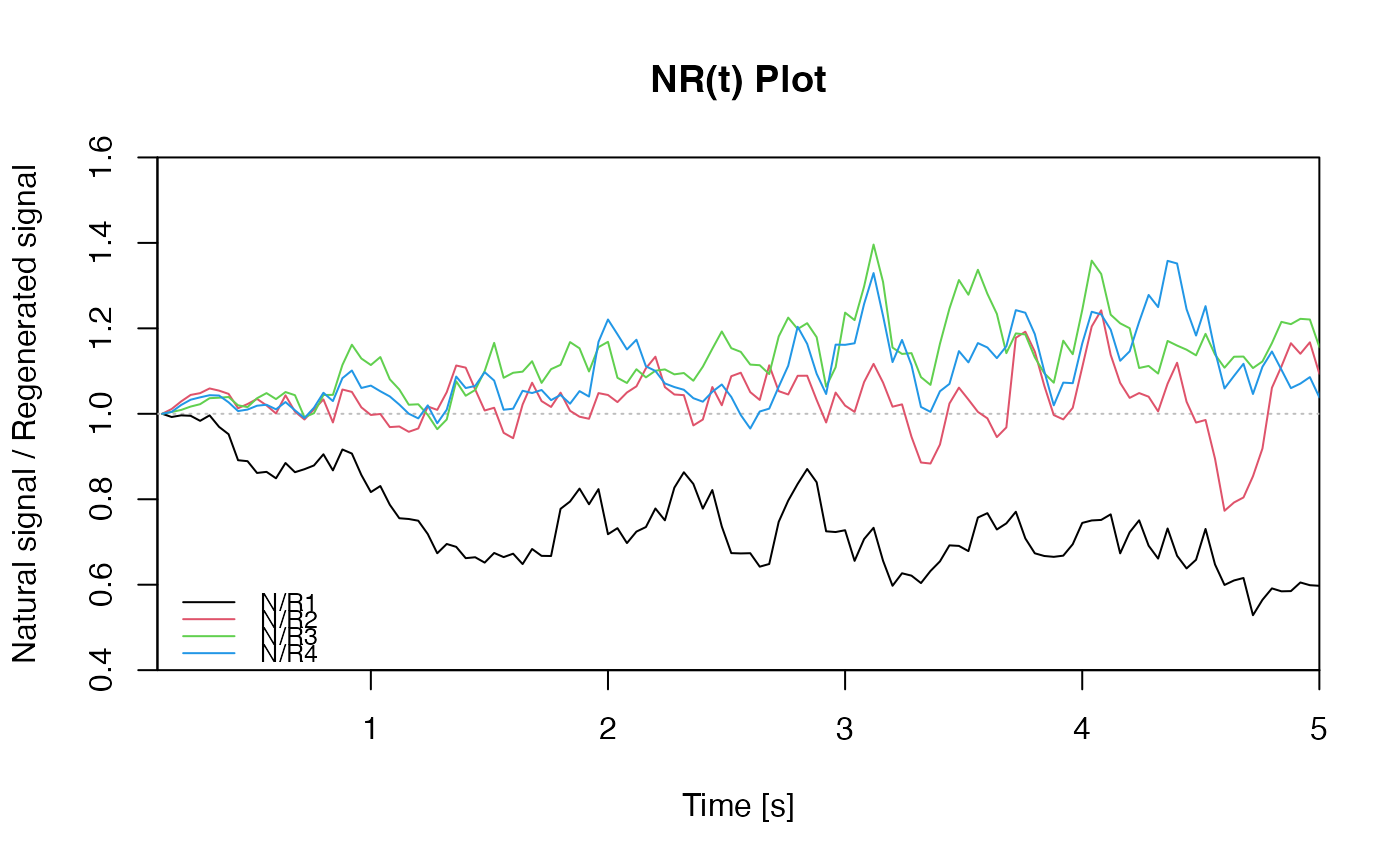
 ## re-plot with custom axes ranges
plot_NRt(curves, smooth = "rmean", k = 5,
xlim = c(0.1, 5), ylim = c(0.4, 1.6),
legend.pos = "bottomleft")
## re-plot with custom axes ranges
plot_NRt(curves, smooth = "rmean", k = 5,
xlim = c(0.1, 5), ylim = c(0.4, 1.6),
legend.pos = "bottomleft")
 ## re-plot with smoothing spline on log scale
plot_NRt(curves, smooth = "spline", log = "x",
legend.pos = "top")
## re-plot with smoothing spline on log scale
plot_NRt(curves, smooth = "spline", log = "x",
legend.pos = "top")
 ## EXAMPLE 2
# you may also use this function to check whether all
# TD curves follow the same shape (making it a TnTx(t) plot).
posTD <- seq(2, 14, 2)
curves <- allCurves[posTD]
plot_NRt(curves, main = "TnTx(t) Plot",
smooth = "rmean", k = 20,
ylab = "TD natural / TD regenerated",
xlim = c(0, 20), legend = FALSE)
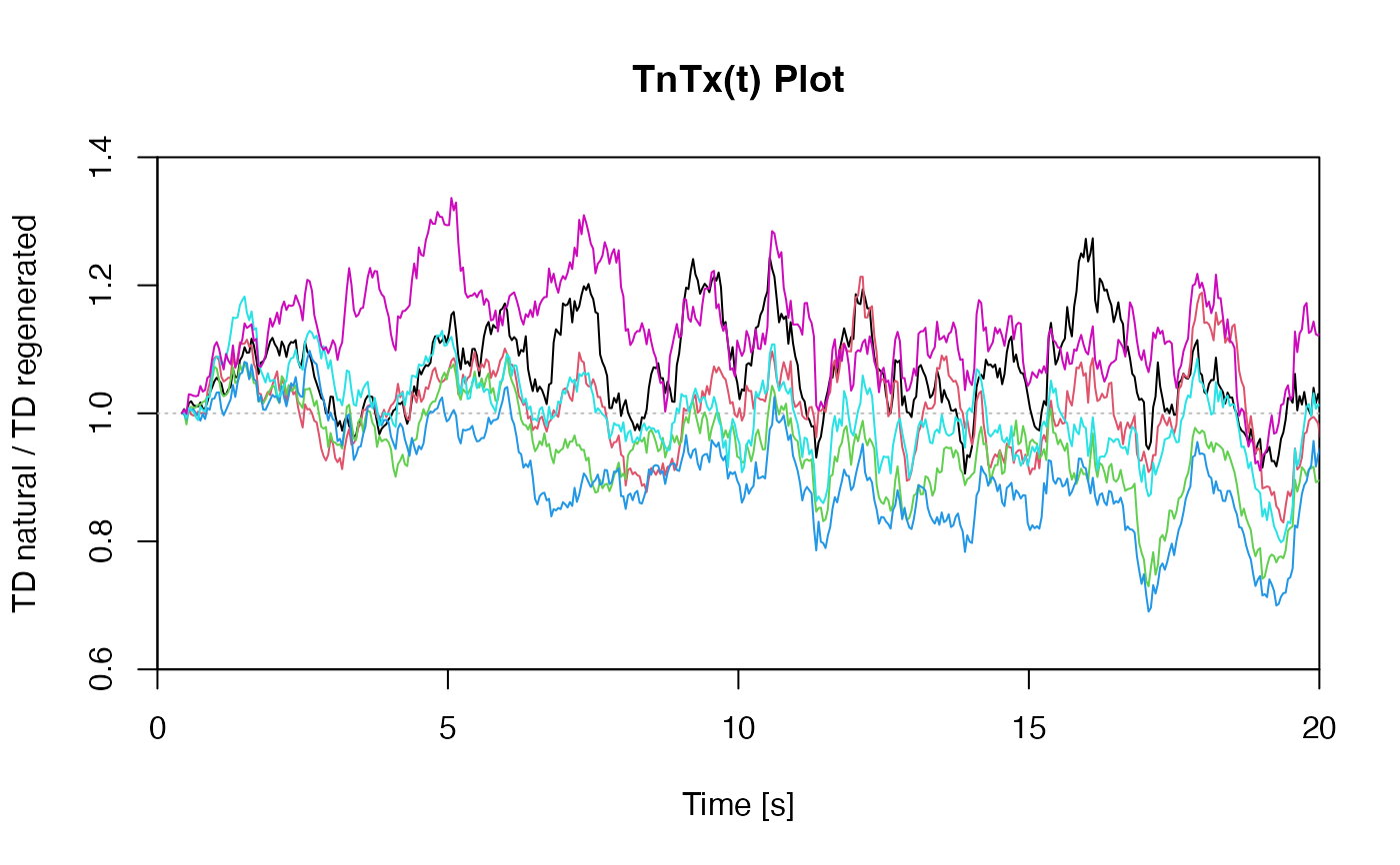
## EXAMPLE 2
# you may also use this function to check whether all
# TD curves follow the same shape (making it a TnTx(t) plot).
posTD <- seq(2, 14, 2)
curves <- allCurves[posTD]
plot_NRt(curves, main = "TnTx(t) Plot",
smooth = "rmean", k = 20,
ylab = "TD natural / TD regenerated",
xlim = c(0, 20), legend = FALSE)
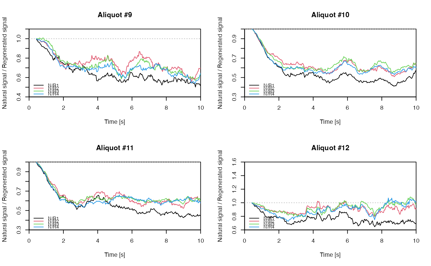
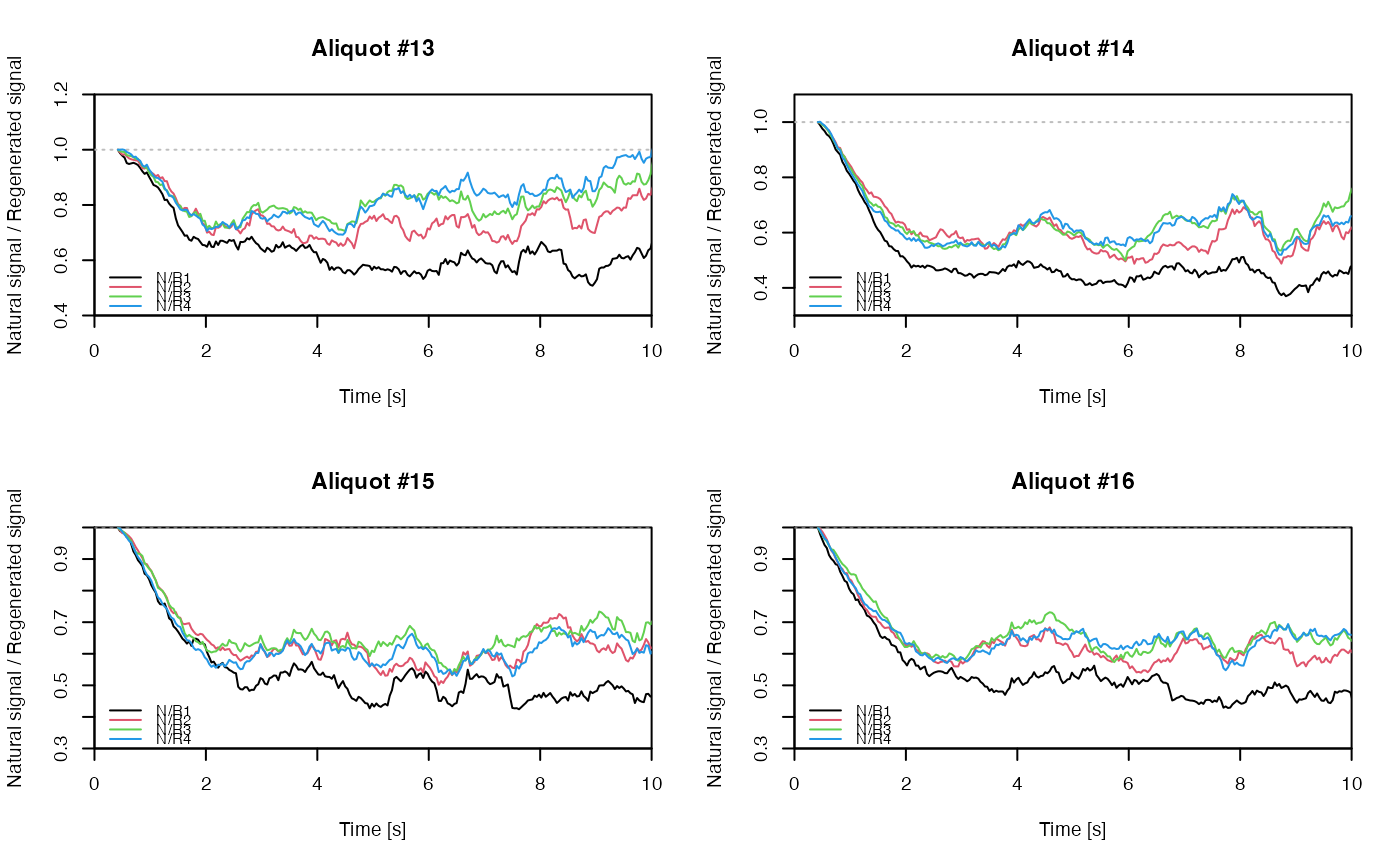
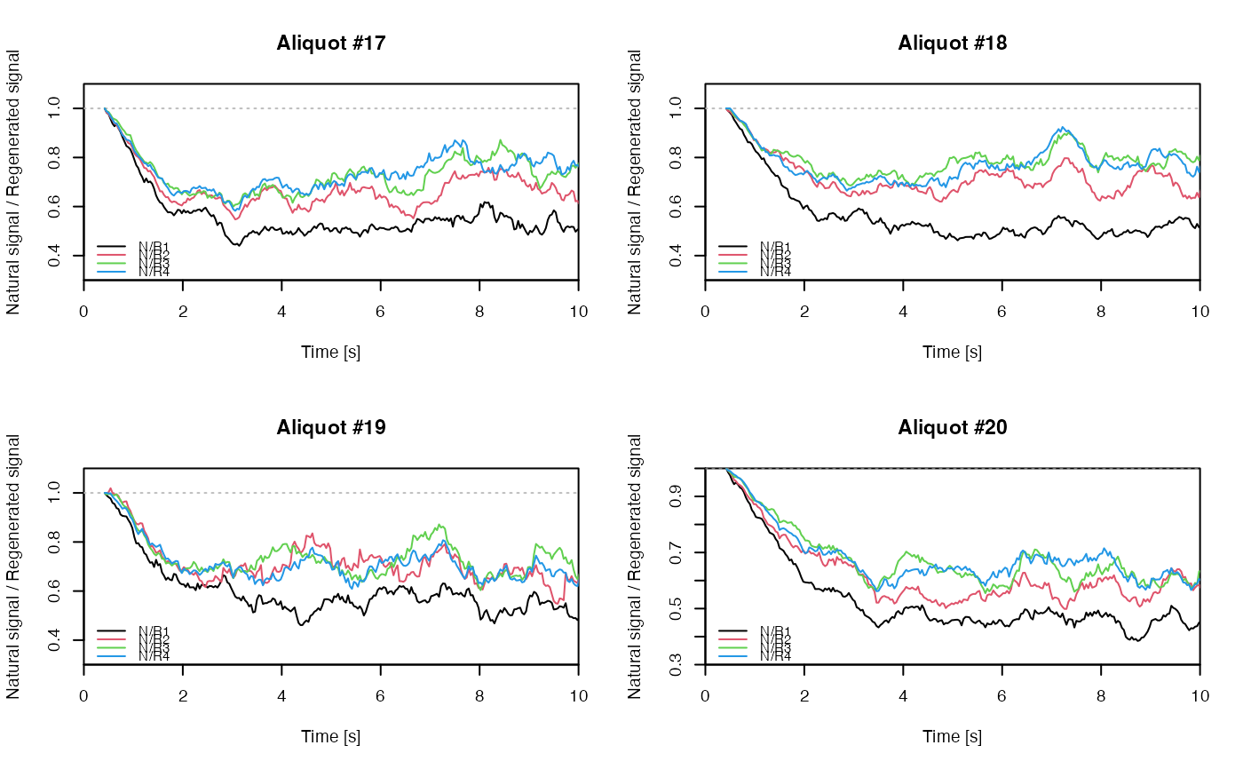
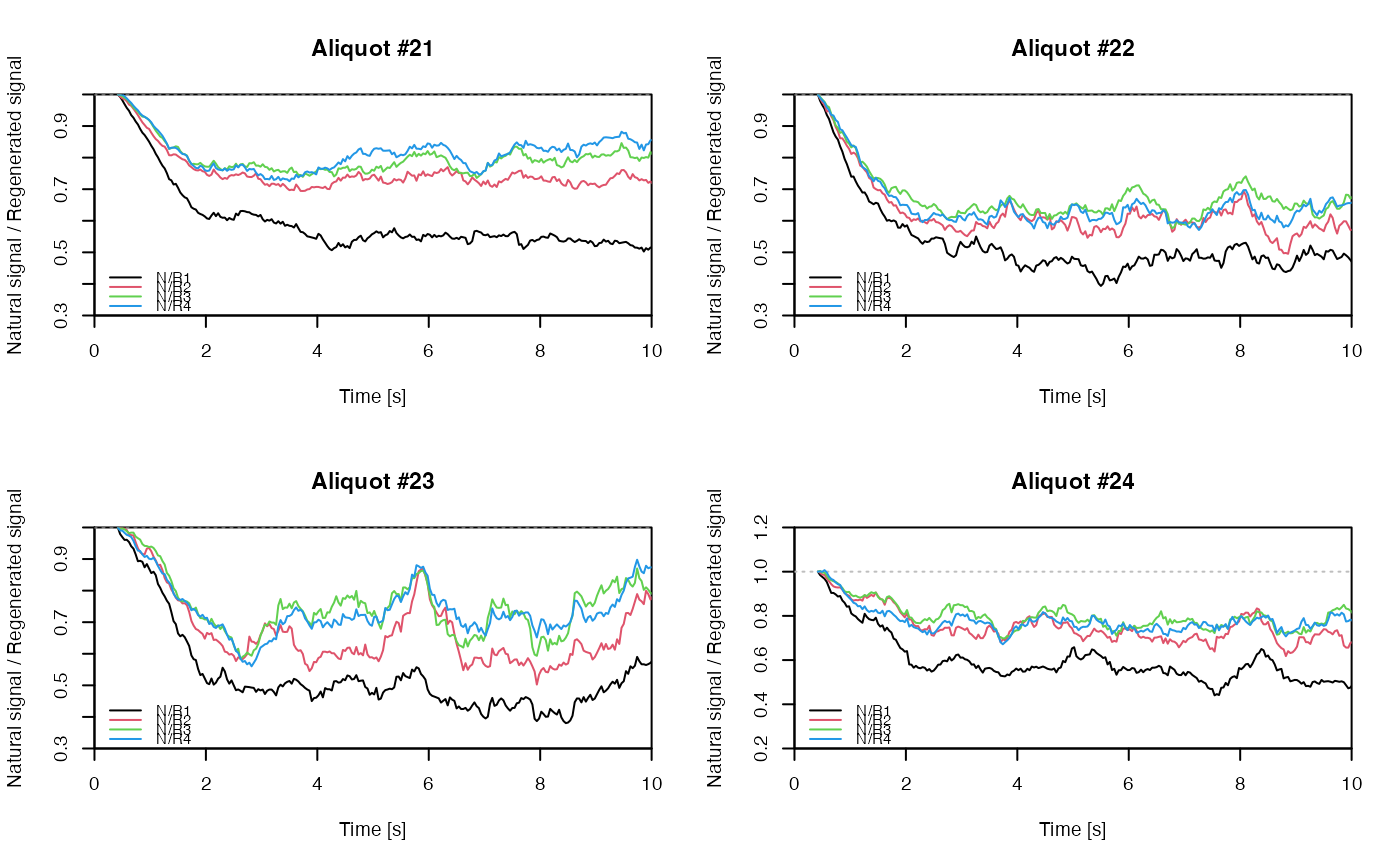
 ## EXAMPLE 3
# extract data from all positions
data <- lapply(1:24, FUN = function(pos) {
Risoe.BINfileData2RLum.Analysis(CWOSL.SAR.Data, pos = pos, ltype = "OSL")
})
# get individual curve data from each aliquot
aliquot <- lapply(data, get_RLum)
# set graphical parameters
par(mfrow = c(2, 2))
# create NR(t) plots for all aliquots
for (i in 1:length(aliquot)) {
plot_NRt(aliquot[[i]][pos],
main = paste0("Aliquot #", i),
smooth = "rmean", k = 20,
xlim = c(0, 10),
cex = 0.6, legend.pos = "bottomleft")
}
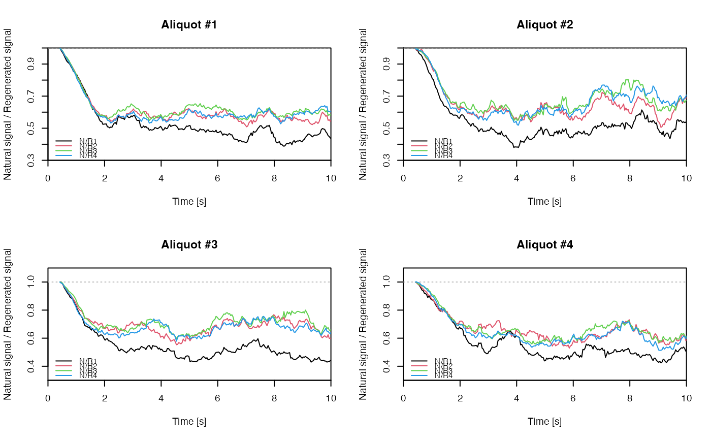
## EXAMPLE 3
# extract data from all positions
data <- lapply(1:24, FUN = function(pos) {
Risoe.BINfileData2RLum.Analysis(CWOSL.SAR.Data, pos = pos, ltype = "OSL")
})
# get individual curve data from each aliquot
aliquot <- lapply(data, get_RLum)
# set graphical parameters
par(mfrow = c(2, 2))
# create NR(t) plots for all aliquots
for (i in 1:length(aliquot)) {
plot_NRt(aliquot[[i]][pos],
main = paste0("Aliquot #", i),
smooth = "rmean", k = 20,
xlim = c(0, 10),
cex = 0.6, legend.pos = "bottomleft")
}
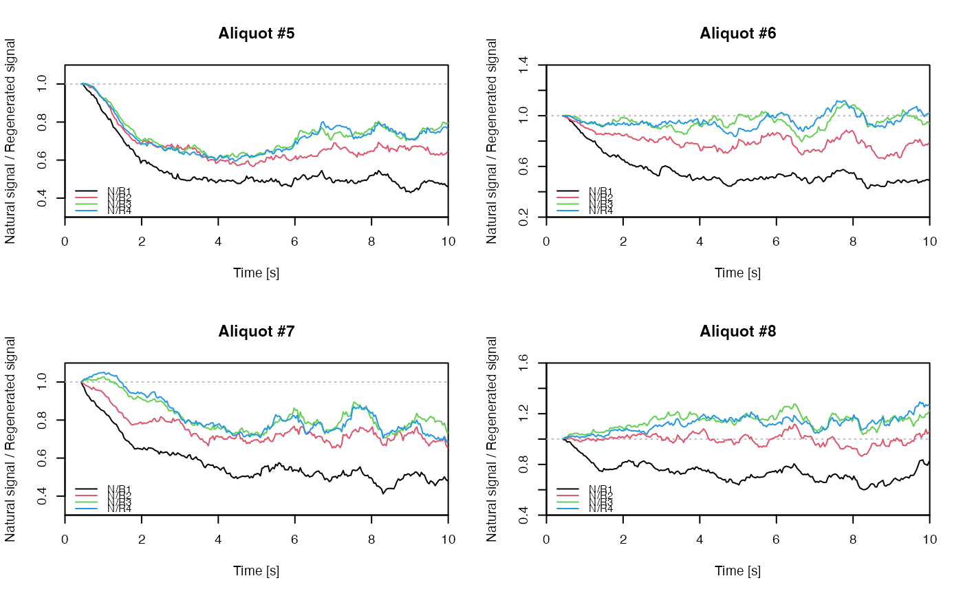

 # reset graphical parameters
par(mfrow = c(1, 1))
# reset graphical parameters
par(mfrow = c(1, 1))