Calculate the gamma dose deposited within a sample accounting for layer-to-layer variations in radioactivity

This function calculates the gamma dose deposited in a luminescence sample taking into account layer-to-layer variations in sediment radioactivity according to Aitken, 1985. The function scales user inputs of uranium, thorium and potassium based on input parameters for sediment density, water content and given layer thicknesses and distances to the sample.

User Input

To calculate the gamma dose deposited in a sample, the user needs to provide sediment information that may influence the luminescence sample. As a rule of thumb, all sediment layers within at least a 30 cm radius from the luminescence sample should be taken into account when calculating the gamma dose rate. However, the actual range of gamma radiation might be different, depending on the emitting radioelements, the water content and the sediment density of each layer (Aitken, 1985). Therefore, the user is advised to provide as much detail as possible that is physically sensible.

The function requires a data.frame with the samples listed in rows. In order, the columns should contain:

Column 1 contains information on the layer/sample ID.
Column 2 gives the thickness (in cm) of each layer.
Column 3: for the layer from which the OSL/TL sample was taken, the distance (in cm) measured from the middle of the sample to the bottom of the layer of interest must be provided. If the whole layer was sampled, insert 0. All layers that are not sampled for OSL/TL should be set to NA.
Columns 4 to 9 contain radionuclide concentrations and their standard errors for potassium (in %), thorium (in ppm) and uranium (in ppm).
Columns 10 and 11 give information on the water content and its standard error in %.
Column 12 contains the layer density (in g/cm³).

No cell should be left blank. Please ensure that the column names match those given in the example dataset, see data('ExampleData.ScaleGammaDose').

The user can decide which dose rate conversion factors should be used to calculate the gamma dose rates. The options are:

"Cresswelletal2018" (Cresswell et al., 2018)
"Liritzisetal2013" (Liritzis et al., 2013)
"Guerinetal2011" (Guérin et al., 2011)
"AdamiecAitken1998" (Adamiec and Aitken, 1998)

Water content

The water content provided by the user should be calculated according to:

$$ \frac{\mathrm{Wet\ weight [g]} - \mathrm{Dry\ weight [g]}} {\mathrm{Dry\ weight [g]}} * 100 $$

Calculations

After converting the radionuclide concentrations into dose rates, the function will scale the dose rates based on the thickness of the layers, the distances to the sample, the water content and the density of the sediment. The calculations are based on Aitken (1985, Appendix H). As an example (equivalent to Aitken, 1985), assuming three layers of sediment, where L is inert and positioned in between the infinite thick and equally active layers A and B, the dose in L and B due to A is given by

$$ {1-f(x)}D_A $$

Where x is the distance into the inert medium, so f(x) is the weighted average fractional dose at x and D_A denotes that the dose is delivered by A. f(x) is derived from table H1 (Aitken, 1985), when setting z = x. Consequently, the dose in A and L due to B is given by

$$ {1 - f(t-x)}D_B $$

Here t is the thickness of L and the other parameters are denoted as above, just for the dose being delivered by B. f(t-x) is derived from table H1 (Aitken, 1985), when setting z equal to t-x. Following this, the dose in L delivered by A and B is given by

$$ {2 - f(x) - f(t-x)}D_{AB} $$

Since A and B are equally active D_{AB} = D_A = D_B.

The function uses the value of the fractional dose rate at the layer boundary to start the calculation for the next layer. This way, the function is able to scale the gamma dose rate accurately for distant layers when the density and water content is not constant for the entire section.

Usage

scale_GammaDose(
  data,
  conversion_factors = c("Cresswelletal2018", "Guerinetal2011", "AdamiecAitken1998",
    "Liritzisetal2013"),
  fractional_gamma_dose = "Aitken1985",
  verbose = TRUE,
  plot = TRUE,
  plot_singlePanels = FALSE,
  ...
)

Arguments

data

data.frame (required): A table containing all relevant information for each individual layer. The table must have the following named columns:

id (character): an arbitrary id or name of each layer
thickness (numeric): vertical extent of each layer in cm
sample_offset (logical): distance of the sample in cm, measured from the bottom of the target layer. Except for the target layer all values must be NA.
K (numeric): K nuclide content in %
K_se (numeric): error on the K content
Th (numeric): Th nuclide content in ppm
Th_se (numeric): error on the Th content
U (numeric): U nuclide content in ppm
U_se (numeric): error on the U content
water_content (numeric): water content of each layer in %
water_content_se (numeric): error on the water content
density (numeric): bulk density of each layer in g/cm^-3

conversion_factors

character (optional): The conversion factors used to calculate the dose rate from sediment nuclide contents. Valid options are:

"Cresswelletal2018" (default)
"Liritzisetal2013"
"Guerinetal2011"
"AdamiecAitken1998"

fractional_gamma_dose

character (optional): Factors to scale gamma dose rate values. Valid options are:

"Aitken1985" (default): Table H1 in the appendix

verbose

logical (with default): enable/disable output to the terminal.

plot

logical (with default): enable/disable the plot output.

plot_singlePanels

logical (with default): enable/disable single plot mode, i.e. one plot window per plot.

...

Further parameters passed to barplot.

Value

After performing the calculations the user is provided with different outputs.

The total gamma dose rate received by the sample (+/- uncertainties) as a print in the console.
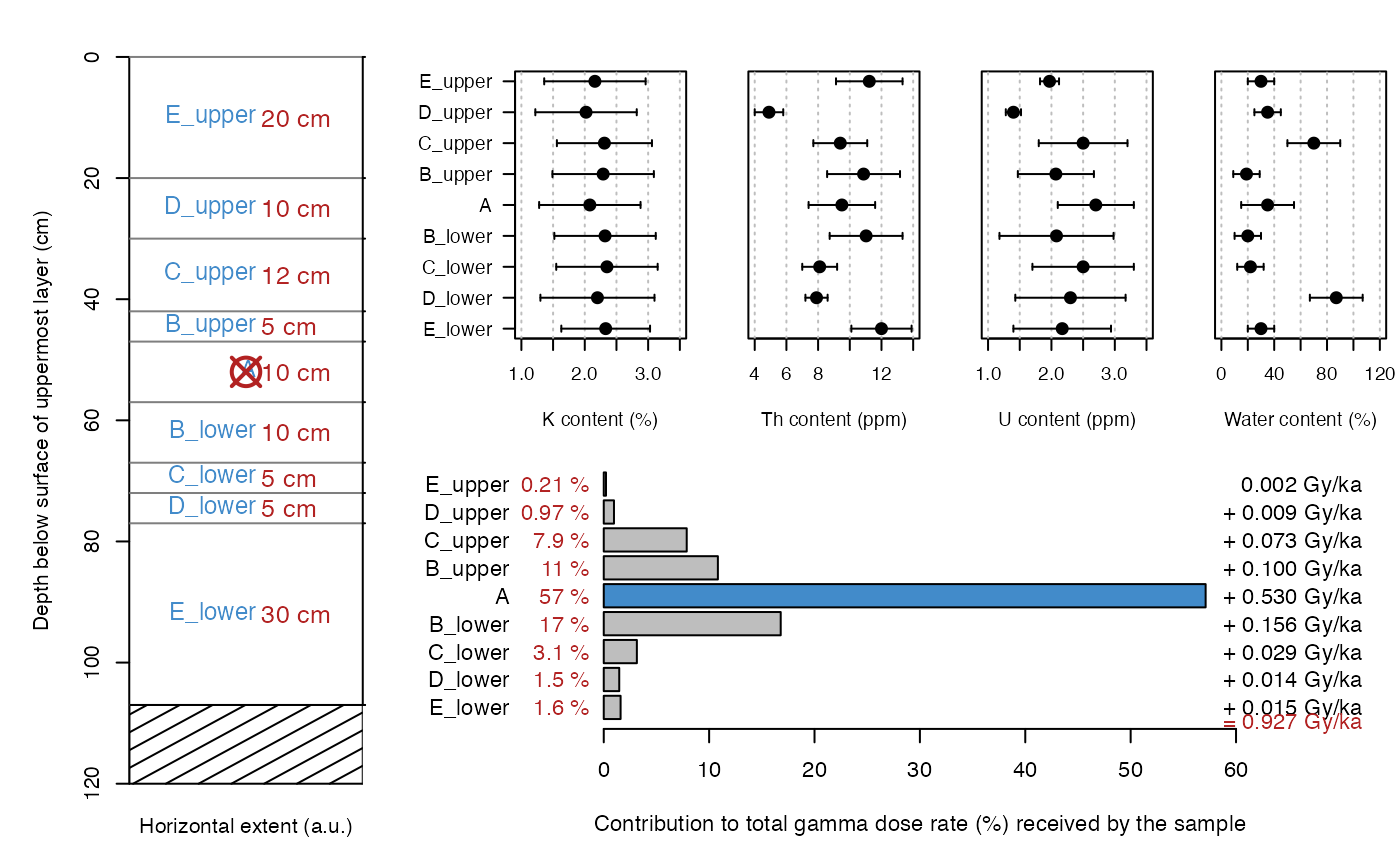
A plot showing the sediment sequence, the user input sample information and the contribution to total gamma dose rate.
RLum Results. If the user wishes to save these results, writing a script to run the function and to save the results would look like this:

mydata <- read.table("c:/path/to/input/file.txt")
results <- scale_GammaDose(mydata)
table <- get_RLum(results)
write.csv(table, "c:/path/to/results.csv")

———————————–
[ NUMERICAL OUTPUT ]
———————————–

RLum.Results-object

slot: @data

Element	Type	Description
`$summary`	`data.frame`	summary of the model results
`$data`	`data.frame`	the original input data
`$dose_rates`	`list`	two `data.frames` for the scaled and infinite matrix dose rates
`$tables`	`list`	several `data.frames` containing intermediate results
`$args`	`character`	arguments of the call
`$call`	`call`	the original function call

slot: @info

Currently unused.

————————
[ PLOT OUTPUT ]
————————

Three plots are produced:

A visualisation of the provided sediment layer structure to quickly assess whether the data was provided and interpreted correctly.
A scatter plot of the nuclide contents per layer (K, Th, U) as well as the water content. This may help to correlate the dose rate contribution of specific layers to the layer of interest.
A barplot visualising the contribution of each layer to the total dose rate received by the sample in the target layer.

Note

This function has BETA status. If possible, results should be cross-checked.

Function version

0.1.4

Acknowledgements

We thank Dr Ian Bailiff for the provision of an excel spreadsheet, which has been very helpful when writing this function.

How to cite

Riedesel, S., Autzen, M., Burow, C., 2026. scale_GammaDose(): Calculate the gamma dose deposited within a sample accounting for layer-to-layer variations in radioactivity. Function version 0.1.4. In: Kreutzer, S., Burow, C., Dietze, M., Fuchs, M.C., Schmidt, C., Fischer, M., Friedrich, J., Mercier, N., Philippe, A., Riedesel, S., Autzen, M., Mittelstrass, D., Gray, H.J., Galharret, J., Colombo, M., Steinbuch, L., de Boer, A., Bluszcz, A., 2026. Luminescence: Comprehensive Luminescence Dating Data Analysis. R package version 1.3.1. https://r-lum.github.io/Luminescence/

References

Aitken, M.J., 1985. Thermoluminescence Dating. Academic Press, London.

Adamiec, G., Aitken, M.J., 1998. Dose-rate conversion factors: update. Ancient TL 16, 37-46. doi:10.26034/la.atl.1998.292

Cresswell., A.J., Carter, J., Sanderson, D.C.W., 2018. Dose rate conversion parameters: Assessment of nuclear data. Radiation Measurements 120, 195-201. doi:10.1016/j.radmeas.2018.02.007

Guérin, G., Mercier, N., Adamiec, G., 2011. Dose-rate conversion factors: update. Ancient TL 29, 5-8. doi:10.26034/la.atl.2011.443

Liritzis, I., Stamoulis, K., Papachristodoulou, C., Ioannides, K., 2013. A re-evaluation of radiation dose-rate conversion factors. Mediterranean Archaeology and Archaeometry 13, 1-15.

Author

Svenja Riedesel, Aberystwyth University (United Kingdom)
Martin Autzen, DTU NUTECH Center for Nuclear Technologies (Denmark)
Christoph Burow, University of Cologne (Germany)
Based on an excel spreadsheet and accompanying macro written by Ian Bailiff. , RLum Developer Team

Examples


# Load example data
data("ExampleData.ScaleGammaDose", envir = environment())

# Scale gamma dose rate
results <- scale_GammaDose(data = ExampleData.ScaleGammaDose,
                           conversion_factors = "Cresswelletal2018",
                           fractional_gamma_dose = "Aitken1985",
                           verbose = TRUE,
                           plot = TRUE)
#> 
#>  [scale_GammaDose()]
#> 
#>  ----
#>  Conversion factors: Cresswelletal2018 
#>  Gamma dose fractions: Aitken1985 
#>  Target layer: A 
#> 
#>  ---- Infinite matrix gamma dose rate per layer ----
#> 
#>        ID   K (Gy/ka)  Th (Gy/ka)   U (Gy/ka) Total (Gy/ka)
#> 1 E_upper 0.399±0.199 0.409±0.156 0.164±0.056         0.973
#> 2 D_upper 0.358±0.175 0.171±0.058 0.112±0.033         0.641
#> 3 C_upper 0.319±0.138 0.256±0.086 0.156±0.062         0.730
#> 4 B_upper 0.467±0.295 0.437±0.248 0.191±0.115         1.094
#> 5       A 0.369±0.254 0.332±0.203 0.216±0.133         0.917
#> 6 B_lower 0.469±0.285 0.439±0.238 0.190±0.125         1.097
#> 7 C_lower 0.466±0.265 0.317±0.150 0.224±0.124         1.006
#> 8 D_lower 0.274±0.129 0.194±0.048 0.129±0.057         0.597
#> 9 E_lower 0.431±0.193 0.437±0.161 0.181±0.088         1.049
#> 
#>  ---- Scaled gamma dose rate for target layer: A  ----
#> 
#>         ID   K (Gy/ka)  Th (Gy/ka)   U (Gy/ka) Contribution (%)
#> 1  E_upper 0.001±0.000 0.001±0.000 0.000±0.000              0.2
#> 2  D_upper 0.005±0.003 0.002±0.001 0.001±0.000              1.0
#> 3  C_upper 0.033±0.014 0.025±0.008 0.015±0.006              7.9
#> 4  B_upper 0.043±0.027 0.040±0.023 0.017±0.010             10.8
#> 5        A 0.207±0.143 0.193±0.118 0.129±0.079             57.1
#> 6  B_lower 0.068±0.041 0.062±0.033 0.026±0.017             16.8
#> 7  C_lower 0.014±0.008 0.009±0.004 0.006±0.003              3.1
#> 8  D_lower 0.007±0.003 0.004±0.001 0.003±0.001              1.5
#> 9  E_lower 0.006±0.003 0.006±0.002 0.002±0.001              1.6
#> 10   TOTAL 0.385±0.152 0.342±0.125 0.200±0.082            100.0
#> 
#>  ----
#>  Infinite matrix gamma dose rate:	 0.917 ± 0.351 Gy/ka 
#>  Scaled gamma dose rate:		 0.927 ± 0.214 Gy/ka
#> 


get_RLum(results)
#>   id dose_rate_K dose_rate_K_err dose_rate_Th dose_rate_Th_err dose_rate_U
#> 1  A   0.3854764       0.1521888    0.3419409        0.1252244   0.1999792
#>   dose_rate_U_err dose_rate_total dose_rate_total_err
#> 1      0.08217342       0.9273965             0.21353