This function models luminescence signals for quartz based on published physical models. It is possible to simulate TL, (CW-) OSL, RF measurements in a arbitrary sequence. This sequence is defined as a list of certain aberrations. Furthermore it is possible to load a sequence direct from the Risø Sequence Editor. The output is an Luminescence::RLum.Analysis object and so the plots are done by the Luminescence::plot_RLum.Analysis function. If a SAR sequence is simulated the plot output can be disabled and SAR analyse functions can be used.
model_LuminescenceSignals(
  model,
  sequence,
  lab.dose_rate = 1,
  simulate_sample_history = FALSE,
  plot = TRUE,
  verbose = TRUE,
  show_structure = FALSE,
  own_parameters = NULL,
  own_state_parameters = NULL,
  own_start_temperature = NULL,
  ...
)
Arguments
- model
character (required): set model to be used. Available models are:
"Bailey2001","Bailey2002","Bailey2004","Pagonis2007","Pagonis2008","Friedrich2017","Friedrich2018","Peng2022" and for own models"customized"(or"customised"). Note: When model ="customized"/"customisedis set, the argumentown_parametershas to be set.- sequence
list (required): set sequence to model as list or as *.seq file from the Risø sequence editor. To simulate SAR measurements there is an extra option to set the sequence list (cf. details).
- lab.dose_rate
numeric (with default): laboratory dose rate in XXX Gy/s for calculating seconds into Gray in the *.seq file.
- simulate_sample_history
logical (with default):
FALSE(with default): simulation begins at laboratory conditions,TRUE: simulations begins at crystallization process (all levels 0)- plot
logical (with default): Enables or disables plot output
- verbose
logical (with default): Verbose mode on/off
- show_structure
logical (with default): Shows the structure of the result. Recommended to show
record.idto analyse concentrations.- own_parameters
list (with default): This argument allows the user to submit own parameter sets. See details for more information.
- own_state_parameters
numeric (with default): Some publications (e.g., Pagonis 2009) offer state parameters. With this argument the user can submit this state parameters. For further details see vignette "RLumModel - Using own parameter sets" and example 3. The parameter also accepts an Luminescence::RLum.Results object created by .set_pars as input.
- own_start_temperature
numeric (with default): Parameter to control the start temperature (in ºC) of a simulation. This parameter takes effect only when 'model = "customized"' is chosen.
- ...
further arguments and graphical parameters passed to plot.default. See details for further information.
Value
This function returns an Luminescence::RLum.Analysis object with all TL, (LM-) OSL and RF/RL steps
in the sequence. Every entry is an Luminescence::RLum.Data.Curve object and can be plotted, analysed etc. with
further RLum-functions.
Details
Defining a sequence
| Arguments | Description | Sub-arguments |
TL | thermally stimulated luminescence | 'temp begin' (ºC), 'temp end' (ºC), 'heating rate' (ºC/s) |
OSL | optically stimulated luminescence | 'temp' (ºC), 'duration' (s), 'optical_power' (%) |
ILL | illumination | 'temp' (ºC), 'duration' (s), 'optical_power' (%) |
LM_OSL | linear modulated OSL | 'temp' (ºC), 'duration' (s), optional: 'start_power' (%), 'end_power' (%) |
RL/RF | radioluminescence | 'temp' (ºC), 'dose' (Gy), 'dose_rate' (Gy/s) |
RF_heating | RF during heating/cooling | 'temp begin' (ºC), 'temp end' (ºC), 'heating rate' (ºC/s], 'dose_rate' (Gy/s) |
IRR | irradiation | 'temp' (ºC), 'dose' (Gy), 'dose_rate' (Gy/s) |
CH | cutheat | 'temp' (ºC), optional: 'duration' (s), 'heating_rate' (ºC/s) |
PH | preheat | 'temp' (ºC), 'duration' (s), optional: 'heating_rate' (ºC/s) |
PAUSE | pause | 'temp' (ºC), 'duration' (s) |
Note: 100% illumination power equates to 20 mW/cm^2
Own parameters
The list has to contain the following items:
N: Concentration of electron- and hole traps (cm^(-3))
E: Electron/Hole trap depth (eV)
s: Frequency factor (s^(-1))
A: Conduction band to electron trap and valence band to hole trap transition probability (s^(-1) * cm^(3)). CAUTION: Not every publication uses the same definition of parameter A and B! See vignette "RLumModel - Usage with own parameter sets" for further details
B: Conduction band to hole centre transition probability (s^(-1) * cm^(3)).
Th: Photo-eviction constant or photoionisation cross section, respectively
E_th: Thermal assistence energy (eV)
k_B: Boltzman constant 8.617e-05 (eV/K)
W: activation energy 0.64 (eV) (for UV)
K: 2.8e7 (dimensionless constant)
model:
"customized"R (optional): Ionisation rate (pair production rate) equivalent to 1 Gy/s (s^(-1)) * cm^(-3))
For further details see Bailey 2001, Wintle 1975, vignette "RLumModel - Using own parameter sets" and example 3.
Defining a SAR-sequence
| Abrivation | Description | examples |
RegDose | Dose points of the regenerative cycles (Gy) | c(0, 80, 140, 260, 320, 0, 80) |
TestDose | Test dose for the SAR cycles (Gy) | 50 |
PH | Temperature of the preheat (ºC) | 240 |
CH | Temperature of the cutheat (ºC) | 200 |
OSL_temp | Temperature of OSL read out (ºC) | 125 |
OSL_duration | Duration of OSL read out (s) | default: 40 |
Irr_temp | Temperature of irradiation (ºC) | default: 20 |
PH_duration | Duration of the preheat (s) | default: 10 |
dose_rate | Dose rate of the laboratory irradiation source (Gy/s) | default: 1 |
optical_power | Percentage of the full illumination power (%) | default: 90 |
Irr_2recover | Dose to be recovered in a dose-recovery-test (Gy) | 20 |
Function version
0.1.6
How to cite
Friedrich, J., Kreutzer, S., 2022. model_LuminescenceSignals(): Model Luminescence Signals. Function version 0.1.6. In: Friedrich, J., Kreutzer, S., Schmidt, C., 2022. RLumModel: Solving Ordinary Differential Equations to Understand Luminescence. R package version 0.2.10. https://CRAN.R-project.org/package=RLumModel
References
Bailey, R.M., 2001. Towards a general kinetic model for optically and thermally stimulated luminescence of quartz. Radiation Measurements 33, 17-45.
Bailey, R.M., 2002. Simulations of variability in the luminescence characteristics of natural quartz and its implications for estimates of absorbed dose. Radiation Protection Dosimetry 100, 33-38.
Bailey, R.M., 2004. Paper I-simulation of dose absorption in quartz over geological timescales and it simplications for the precision and accuracy of optical dating. Radiation Measurements 38, 299-310.
Friedrich, J., Kreutzer, S., Schmidt, C., 2016. Solving ordinary differential equations to understand luminescence: 'RLumModel', an advanced research tool for simulating luminescence in quartz using R. Quaternary Geochronology 35, 88-100.
Friedrich, J., Pagonis, V., Chen, R., Kreutzer, S., Schmidt, C., 2017: Quartz radiofluorescence: a modelling approach. Journal of Luminescence 186, 318-325.
Pagonis, V., Chen, R., Wintle, A.G., 2007: Modelling thermal transfer in optically stimulated luminescence of quartz. Journal of Physics D: Applied Physics 40, 998-1006.
Pagonis, V., Wintle, A.G., Chen, R., Wang, X.L., 2008. A theoretical model for a new dating protocol for quartz based on thermally transferred OSL (TT-OSL). Radiation Measurements 43, 704-708.
Pagonis, V., Lawless, J., Chen, R., Anderson, C., 2009. Radioluminescence in Al2O3:C - analytical and numerical simulation results. Journal of Physics D: Applied Physics 42, 175107 (9pp).
Peng, J., Wang, X., Adamiec, G., 2022. The build-up of the laboratory-generated dose-response curve and underestimation of equivalent dose for quartz OSL in the high dose region: A critical modelling study. Quaternary Geochronology 67, 101231.
Soetaert, K., Cash, J., Mazzia, F., 2012. Solving differential equations in R. Springer Science & Business Media.
Wintle, A., 1975. Thermal Quenching of Thermoluminescence in Quartz. Geophysical Journal International 41, 107-113.
See also
Examples
##================================================================##
## Example 1: Simulate Bailey2001
## (cf. Bailey, 2001, Fig. 1)
##================================================================##
##set sequence with the following steps
## (1) Irradiation at 20 deg. C with a dose of 10 Gy and a dose rate of 1 Gy/s
## (2) TL from 20-400 deg. C with a rate of 5 K/s
sequence <-
list(
IRR = c(20, 10, 1),
TL = c(20, 400, 5)
)
##model sequence
model.output <- model_LuminescenceSignals(
sequence = sequence,
model = "Bailey2001"
)
#>
#> [.translate_Sequence()]
#> >> Simulate sequence
#>
|
| | 0%
|
|=================================== | 50%
|
|======================================================================| 100%
 ##get all TL concentrations
TL_conc <- get_RLum(model.output, recordType = "(TL)", drop = FALSE)
plot_RLum(TL_conc)
##get all TL concentrations
TL_conc <- get_RLum(model.output, recordType = "(TL)", drop = FALSE)
plot_RLum(TL_conc)

 ##plot 110 deg. C trap concentration
TL_110 <- get_RLum(TL_conc, recordType = "conc. level 1")
plot_RLum(TL_110)
##plot 110 deg. C trap concentration
TL_110 <- get_RLum(TL_conc, recordType = "conc. level 1")
plot_RLum(TL_110)
 ##============================================================================##
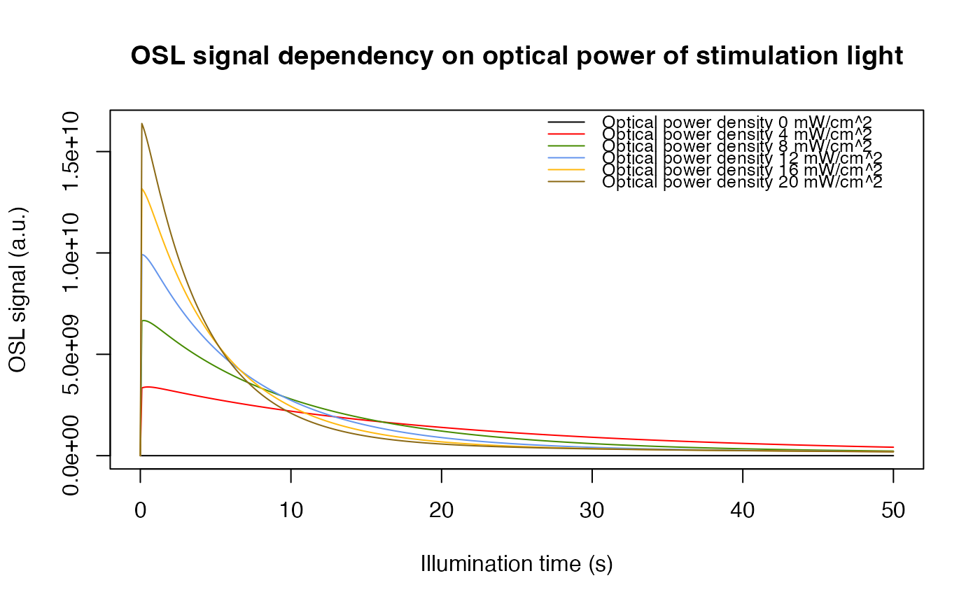
## Example 2: compare different optical powers of stimulation light
##============================================================================##
# call function "model_LuminescenceSignals", model = "Bailey2004"
# and simulate_sample_history = FALSE (default),
# because the sample history is not part of the sequence
# the optical_power of the LED is varied and then compared.
optical_power <- seq(from = 0,to = 100,by = 20)
model.output <- lapply(optical_power, function(x){
sequence <- list(IRR = c(20, 50, 1),
PH = c(220, 10, 5),
OSL = c(125, 50, x)
)
data <- model_LuminescenceSignals(
sequence = sequence,
model = "Bailey2004",
plot = FALSE,
verbose = FALSE
)
return(get_RLum(data, recordType = "OSL$", drop = FALSE))
})
##combine output curves
model.output.merged <- merge_RLum(model.output)
##plot
plot_RLum(
object = model.output.merged,
xlab = "Illumination time (s)",
ylab = "OSL signal (a.u.)",
main = "OSL signal dependency on optical power of stimulation light",
legend.text = paste("Optical power density", 20*optical_power/100, "mW/cm^2"),
combine = TRUE)
##============================================================================##
## Example 2: compare different optical powers of stimulation light
##============================================================================##
# call function "model_LuminescenceSignals", model = "Bailey2004"
# and simulate_sample_history = FALSE (default),
# because the sample history is not part of the sequence
# the optical_power of the LED is varied and then compared.
optical_power <- seq(from = 0,to = 100,by = 20)
model.output <- lapply(optical_power, function(x){
sequence <- list(IRR = c(20, 50, 1),
PH = c(220, 10, 5),
OSL = c(125, 50, x)
)
data <- model_LuminescenceSignals(
sequence = sequence,
model = "Bailey2004",
plot = FALSE,
verbose = FALSE
)
return(get_RLum(data, recordType = "OSL$", drop = FALSE))
})
##combine output curves
model.output.merged <- merge_RLum(model.output)
##plot
plot_RLum(
object = model.output.merged,
xlab = "Illumination time (s)",
ylab = "OSL signal (a.u.)",
main = "OSL signal dependency on optical power of stimulation light",
legend.text = paste("Optical power density", 20*optical_power/100, "mW/cm^2"),
combine = TRUE)
 ##============================================================================##
## Example 3: Usage of own parameter sets (Pagonis 2009)
##============================================================================##
own_parameters <- list(
N = c(2e15, 2e15, 1e17, 2.4e16),
E = c(0, 0, 0, 0),
s = c(0, 0, 0, 0),
A = c(2e-8, 2e-9, 4e-9, 1e-8),
B = c(0, 0, 5e-11, 4e-8),
Th = c(0, 0),
E_th = c(0, 0),
k_B = 8.617e-5,
W = 0.64,
K = 2.8e7,
model = "customized",
R = 1.7e15
)
## Note: In Pagonis 2009 is B the valence band to hole centre probability,
## but in Bailey 2001 this is A_j. So the values of B (in Pagonis 2009)
## are A in the notation above. Also notice that the first two entries in N, A and
## B belong to the electron traps and the last two entries to the hole centres.
own_state_parameters <- c(0, 0, 0, 9.4e15)
## calculate Fig. 3 in Pagonis 2009. Note: The labels for the dose rate in the original
## publication are not correct.
## For a dose rate of 0.1 Gy/s belongs a RF signal to ~ 1.5e14 (see Fig. 6).
sequence <- list(RF = c(20, 0.1, 0.1))
model_LuminescenceSignals(
model = "customized",
sequence = sequence,
own_parameters = own_parameters,
own_state_parameters = own_state_parameters)
#>
#> [.translate_Sequence()]
#> >> Simulate sequence
#>
|
| | 0%
|
|======================================================================| 100%
##============================================================================##
## Example 3: Usage of own parameter sets (Pagonis 2009)
##============================================================================##
own_parameters <- list(
N = c(2e15, 2e15, 1e17, 2.4e16),
E = c(0, 0, 0, 0),
s = c(0, 0, 0, 0),
A = c(2e-8, 2e-9, 4e-9, 1e-8),
B = c(0, 0, 5e-11, 4e-8),
Th = c(0, 0),
E_th = c(0, 0),
k_B = 8.617e-5,
W = 0.64,
K = 2.8e7,
model = "customized",
R = 1.7e15
)
## Note: In Pagonis 2009 is B the valence band to hole centre probability,
## but in Bailey 2001 this is A_j. So the values of B (in Pagonis 2009)
## are A in the notation above. Also notice that the first two entries in N, A and
## B belong to the electron traps and the last two entries to the hole centres.
own_state_parameters <- c(0, 0, 0, 9.4e15)
## calculate Fig. 3 in Pagonis 2009. Note: The labels for the dose rate in the original
## publication are not correct.
## For a dose rate of 0.1 Gy/s belongs a RF signal to ~ 1.5e14 (see Fig. 6).
sequence <- list(RF = c(20, 0.1, 0.1))
model_LuminescenceSignals(
model = "customized",
sequence = sequence,
own_parameters = own_parameters,
own_state_parameters = own_state_parameters)
#>
#> [.translate_Sequence()]
#> >> Simulate sequence
#>
|
| | 0%
|
|======================================================================| 100%
 #>
#> [RLum.Analysis-class]
#> originator: model_LuminescenceSignals()
#> protocol: customized
#> additional info elements: 3
#> number of records: 7
#> .. : RLum.Data.Curve : 7
#> .. .. : #1 RF | #2 conc. level 1 (RF) | #3 conc. level 2 (RF) | #4 conc. level 3 (RF) | #5 conc. level 4 (RF) | #6 conc. n_c (RF) | #7 conc. n_v (RF)
if (FALSE) {
##============================================================================##
## Example 4: Simulate Thermal-Activation-Characteristics (TAC)
##============================================================================##
##set temperature
act.temp <- seq(from = 80, to = 600, by = 20)
##loop over temperature
model.output <- vapply(X = act.temp, FUN = function(x) {
##set sequence, note: sequence includes sample history
sequence <- list(
IRR = c(20, 1, 1e-11),
IRR = c(20, 10, 1),
PH = c(x, 1),
IRR = c(20, 0.1, 1),
TL = c(20, 150, 5)
)
##run simulation
temp <- model_LuminescenceSignals(
sequence = sequence,
model = "Pagonis2007",
simulate_sample_history = TRUE,
plot = FALSE,
verbose = FALSE
)
## "TL$" for exact matching TL and not (TL)
TL_curve <- get_RLum(temp, recordType = "TL$")
##return max value in TL curve
return(max(get_RLum(TL_curve)[,2]))
}, FUN.VALUE = 1)
##plot resutls
plot(
act.temp[-(1:3)],
model.output[-(1:3)],
type = "b",
xlab = "Temperature [\u00B0C)",
ylab = "TL [a.u.]"
)
##============================================================================##
## Example 5: Simulate SAR sequence
##============================================================================##
##set SAR sequence with the following steps
## (1) RegDose: set regenerative dose (Gy) as vector
## (2) TestDose: set test dose (Gy)
## (3) PH: set preheat temperature in deg. C
## (4) CH: Set cutheat temperature in deg. C
## (5) OSL_temp: set OSL reading temperature in deg. C
## (6) OSL_duration: set OSL reading duration in s
sequence <- list(
RegDose = c(0,10,20,50,90,0,10),
TestDose = 5,
PH = 240,
CH = 200,
OSL_temp = 125,
OSL_duration = 70)
# call function "model_LuminescenceSignals", set sequence = sequence,
# model = "Pagonis2007" (palaeodose = 20 Gy) and simulate_sample_history = FALSE (default),
# because the sample history is not part of the sequence
model.output <- model_LuminescenceSignals(
sequence = sequence,
model = "Pagonis2007",
plot = FALSE
)
# in environment is a new object "model.output" with the results of
# every step of the given sequence.
# Plots are done at OSL and TL steps and the growth curve
# call "analyse_SAR.CWOSL" from RLum package
results <- analyse_SAR.CWOSL(model.output,
signal.integral.min = 1,
signal.integral.max = 15,
background.integral.min = 601,
background.integral.max = 701,
fit.method = "EXP",
dose.points = c(0,10,20,50,90,0,10))
##============================================================================##
## Example 6: generate sequence from *.seq file and run SAR simulation
##============================================================================##
# load example *.SEQ file and construct a sequence.
# call function "model_LuminescenceSignals", load created sequence for sequence,
# set model = "Bailey2002" (palaeodose = 10 Gy)
# and simulate_sample_history = FALSE (default),
# because the sample history is not part of the sequence
path <- system.file("extdata", "example_SAR_cycle.SEQ", package="RLumModel")
sequence <- read_SEQ2R(file = path)
model.output <- model_LuminescenceSignals(
sequence = sequence,
model = "Bailey2001",
plot = FALSE
)
## call RLum package function "analyse_SAR.CWOSL" to analyse the simulated SAR cycle
results <- analyse_SAR.CWOSL(model.output,
signal.integral.min = 1,
signal.integral.max = 10,
background.integral.min = 301,
background.integral.max = 401,
dose.points = c(0,8,14,26,32,0,8),
fit.method = "EXP")
print(get_RLum(results))
##============================================================================##
## Example 7: Simulate sequence at laboratory without sample history
##============================================================================##
##set sequence with the following steps
## (1) Irraditation at 20 deg. C with a dose of 100 Gy and a dose rate of 1 Gy/s
## (2) Preheat to 200 deg. C and hold for 10 s
## (3) LM-OSL at 125 deg. C. for 100 s
## (4) Cutheat at 200 dec. C.
## (5) Irraditation at 20 deg. C with a dose of 10 Gy and a dose rate of 1 Gy/s
## (6) Pause at 200 de. C. for 100 s
## (7) OSL at 125 deg. C for 100 s with 90 % optical power
## (8) Pause at 200 deg. C for 100 s
## (9) TL from 20-400 deg. C with a heat rate of 5 K/s
## (10) Radiofluorescence at 20 deg. C with a dose of 200 Gy and a dose rate of 0.01 Gy/s
sequence <-
list(
IRR = c(20, 100, 1),
PH = c(200, 10),
LM_OSL = c(125, 100),
CH = c(200),
IRR = c(20, 10, 1),
PAUSE = c(200, 100),
OSL = c(125, 100, 90),
PAUSE = c(200, 100),
TL = c(20, 400, 5),
RF = c(20, 200, 0.01)
)
# call function "model_LuminescenceSignals", set sequence = sequence,
# model = "Pagonis2008" (palaeodose = 200 Gy) and simulate_sample_history = FALSE (default),
# because the sample history is not part of the sequence
model.output <- model_LuminescenceSignals(
sequence = sequence,
model = "Pagonis2008"
)
}
#>
#> [RLum.Analysis-class]
#> originator: model_LuminescenceSignals()
#> protocol: customized
#> additional info elements: 3
#> number of records: 7
#> .. : RLum.Data.Curve : 7
#> .. .. : #1 RF | #2 conc. level 1 (RF) | #3 conc. level 2 (RF) | #4 conc. level 3 (RF) | #5 conc. level 4 (RF) | #6 conc. n_c (RF) | #7 conc. n_v (RF)
if (FALSE) {
##============================================================================##
## Example 4: Simulate Thermal-Activation-Characteristics (TAC)
##============================================================================##
##set temperature
act.temp <- seq(from = 80, to = 600, by = 20)
##loop over temperature
model.output <- vapply(X = act.temp, FUN = function(x) {
##set sequence, note: sequence includes sample history
sequence <- list(
IRR = c(20, 1, 1e-11),
IRR = c(20, 10, 1),
PH = c(x, 1),
IRR = c(20, 0.1, 1),
TL = c(20, 150, 5)
)
##run simulation
temp <- model_LuminescenceSignals(
sequence = sequence,
model = "Pagonis2007",
simulate_sample_history = TRUE,
plot = FALSE,
verbose = FALSE
)
## "TL$" for exact matching TL and not (TL)
TL_curve <- get_RLum(temp, recordType = "TL$")
##return max value in TL curve
return(max(get_RLum(TL_curve)[,2]))
}, FUN.VALUE = 1)
##plot resutls
plot(
act.temp[-(1:3)],
model.output[-(1:3)],
type = "b",
xlab = "Temperature [\u00B0C)",
ylab = "TL [a.u.]"
)
##============================================================================##
## Example 5: Simulate SAR sequence
##============================================================================##
##set SAR sequence with the following steps
## (1) RegDose: set regenerative dose (Gy) as vector
## (2) TestDose: set test dose (Gy)
## (3) PH: set preheat temperature in deg. C
## (4) CH: Set cutheat temperature in deg. C
## (5) OSL_temp: set OSL reading temperature in deg. C
## (6) OSL_duration: set OSL reading duration in s
sequence <- list(
RegDose = c(0,10,20,50,90,0,10),
TestDose = 5,
PH = 240,
CH = 200,
OSL_temp = 125,
OSL_duration = 70)
# call function "model_LuminescenceSignals", set sequence = sequence,
# model = "Pagonis2007" (palaeodose = 20 Gy) and simulate_sample_history = FALSE (default),
# because the sample history is not part of the sequence
model.output <- model_LuminescenceSignals(
sequence = sequence,
model = "Pagonis2007",
plot = FALSE
)
# in environment is a new object "model.output" with the results of
# every step of the given sequence.
# Plots are done at OSL and TL steps and the growth curve
# call "analyse_SAR.CWOSL" from RLum package
results <- analyse_SAR.CWOSL(model.output,
signal.integral.min = 1,
signal.integral.max = 15,
background.integral.min = 601,
background.integral.max = 701,
fit.method = "EXP",
dose.points = c(0,10,20,50,90,0,10))
##============================================================================##
## Example 6: generate sequence from *.seq file and run SAR simulation
##============================================================================##
# load example *.SEQ file and construct a sequence.
# call function "model_LuminescenceSignals", load created sequence for sequence,
# set model = "Bailey2002" (palaeodose = 10 Gy)
# and simulate_sample_history = FALSE (default),
# because the sample history is not part of the sequence
path <- system.file("extdata", "example_SAR_cycle.SEQ", package="RLumModel")
sequence <- read_SEQ2R(file = path)
model.output <- model_LuminescenceSignals(
sequence = sequence,
model = "Bailey2001",
plot = FALSE
)
## call RLum package function "analyse_SAR.CWOSL" to analyse the simulated SAR cycle
results <- analyse_SAR.CWOSL(model.output,
signal.integral.min = 1,
signal.integral.max = 10,
background.integral.min = 301,
background.integral.max = 401,
dose.points = c(0,8,14,26,32,0,8),
fit.method = "EXP")
print(get_RLum(results))
##============================================================================##
## Example 7: Simulate sequence at laboratory without sample history
##============================================================================##
##set sequence with the following steps
## (1) Irraditation at 20 deg. C with a dose of 100 Gy and a dose rate of 1 Gy/s
## (2) Preheat to 200 deg. C and hold for 10 s
## (3) LM-OSL at 125 deg. C. for 100 s
## (4) Cutheat at 200 dec. C.
## (5) Irraditation at 20 deg. C with a dose of 10 Gy and a dose rate of 1 Gy/s
## (6) Pause at 200 de. C. for 100 s
## (7) OSL at 125 deg. C for 100 s with 90 % optical power
## (8) Pause at 200 deg. C for 100 s
## (9) TL from 20-400 deg. C with a heat rate of 5 K/s
## (10) Radiofluorescence at 20 deg. C with a dose of 200 Gy and a dose rate of 0.01 Gy/s
sequence <-
list(
IRR = c(20, 100, 1),
PH = c(200, 10),
LM_OSL = c(125, 100),
CH = c(200),
IRR = c(20, 10, 1),
PAUSE = c(200, 100),
OSL = c(125, 100, 90),
PAUSE = c(200, 100),
TL = c(20, 400, 5),
RF = c(20, 200, 0.01)
)
# call function "model_LuminescenceSignals", set sequence = sequence,
# model = "Pagonis2008" (palaeodose = 200 Gy) and simulate_sample_history = FALSE (default),
# because the sample history is not part of the sequence
model.output <- model_LuminescenceSignals(
sequence = sequence,
model = "Pagonis2008"
)
}