RLumModel - Getting started with RLumModel
Johannes Friedrich (University of Bayreuth, DE) & Sebastian Kreutzer (Geography and Earth Sciences, Aberystwyth University, UK)
2022-02-20
Source:vignettes/RLumModel_-_Getting_started_with_RLumModel.Rmd
RLumModel_-_Getting_started_with_RLumModel.RmdIntroduction
This vignette shows a few examples for the R-package
‘RLumModel’. The main function model_LuminescenceSignals()
and their arguments will be explained. All calculations were done with
‘RLumModel’ (version: 0.2.10) and ‘Luminescence’ (version:
0.9.19.9000.7).
Object structure of RLumModel
The output from the main function
model_LuminescenceSignals() is of class
RLum.Analysis (Kreutzer et al.
2012) and contains data of class RLum.Data.Curve in
the slot ‘records’. The advantage of this infrastructure is that the
package ‘Luminescence’ offers a lot of methods to visualize and
manipulate data.
All simulated data are stored in the slot ‘records’: TL/OSL/RF curves as well as the concentrations of every energy level from every step.
The following code loads a data set provided by the ‘RLumModel’ package and shows how to separate TL/OSL/RF data from concentrations and how to visualize them.
data("ExampleData.ModelOutput", package = "RLumModel")

##show class
class(model.output)

##show structure
Luminescence::structure_RLum(model.output)

##separate TL-curve from TL-concentrations
TL_curve <- Luminescence::get_RLum(model.output, recordType = "TL$")
TL_conc <- Luminescence::get_RLum(model.output, recordType = "(TL)", drop = FALSE)

##also possible: TL_curve <- get_RLum(model.output, record.id = 1)

##plot results
Luminescence::plot_RLum(TL_curve)
Luminescence::plot_RLum(TL_conc)
Some notes to the code example above:
- in ‘TL_curve <- …’ appears “TL$”. This is necessary to match the pattern “TL” without any sign after “TL”, e.g. a bracket. The brackets are used (by default) for the concentrations.
- in ‘TL_conc <- …’ the pattern “(TL)” will match all concentrations with “(TL)”, see structure.
-
drop = FALSEwas used to keep theRLum.Analysisclass for ‘TL_conc’. - To see a single plot of every energy-level, use the option
plot.single = TRUEinplot_RLum(). For more details see the manual of ‘Luminescence’.
##plot every energy-level by an extra plot
Luminescence::plot_RLum(TL_conc, plot.single = TRUE)
It is also possible to choose a RLum.Data.Curve by their
‘record.id’, which can be seen with:
##see structure of model.output
Luminescence::structure_RLum(model.output)
Selecting a quartz luminescence model
The first argument required for the function
model_LuminescenceSignals() is the name of a quartz
luminescence model to be used, respectively the used parameter set in
this quartz luminescence model. All currently implemented quartz
luminescence models were described in Friedrich,
Kreutzer, and Schmidt (2016). The command to select a set of
parameters from a specific model in RLumModel is a
character string with the name of the author and the year, e.g.
model <- "Bailey2001"The available models are “Bailey2001”, “Bailey2002”, “Bailey2004”, “Pagonis2007”, “Pagonis2008”,“Friedrich2017” and “customized” (R. M. Bailey (2001), R. Bailey (2002), R. Bailey (2004), V. Pagonis, Chen, and Wintle (2007), V. Pagonis et al. (2008b), Friedrich et al. (2017)). For customized or own parameter sets, see vignette RLumModel - Using own parameter sets
The corresponding parameter set will be loaded automatically with the function call.
Creating a sequence
The second argument in the model_LuminescenceSignals()
function is the sequence to be simulated. There are three different ways
of creating a sequence.
For all sequences, temperature differences between sequence steps are automatically simulated with a heating or cooling step in between. Also, after irradiating the sample, it is automatically kept at irradiation temperature for further 5 s to allow the system to relax prior to the next step (R. M. Bailey 2001).
Risø SEQ files
The first one is to use the popular and freely available Risø to build a personal sequence and to save it as a SEQ-file (*.seq). Files created by the Sequence Editor can be imported directly using the path of the SEQ-file. The package comes along with an example SEQ-file in the package folder in ‘extdata’. Thus, a potential sequence is created with
sequence <- system.file(
  "extdata",
  "example_SAR_cycle.SEQ",
  package = "RLumModel")
or wherever the SEQ-file is stored. While in the Sequence Editor
irradiation is commonly defined in seconds, performing the simulation
requires a dose transformation to Gray. Therefore, the function
model_LuminescenceSignals() offers a special argument
called lab.dose_rate, representing the dose rate of the
irradiation unit in the laboratory. By default, this dose rate is 1
Gy/s, but can be modified, e.g.,
lab.dose_rate <- 0.105Keywords
The second way of creating a sequence is by referring to a list with
keywords and a certain order of code numbers or named values, which are
shown in Table 1. With these keywords, it is possible to create quickly
an R object of type list, which can be read by the
model_LuminescenceSignals() function.
| ARGUMENTS | DESCRIPTION | SUB-ARGUMENTS |
|---|---|---|
| TL | Thermally stimulated luminescence | ’temp_begin’ [°C], ’temp_end’ [°C], ’heating_rate’ [°C/s] |
| OSL | Optically stimulated luminescence | ’temp’ [°C], ’duration’ [s], ’optical_power’ [%] |
| ILL | Illumination | ’temp’ [°C], ’duration’ [s], ’optical_power’ [%] |
| LM_OSL | Linear modulated OSL | ’temp’ [°C], ’duration’ [s], optional: ’start_power’ [%], ’end_power’ [%] |
| RF | Radiofluorescence | ’temp’ [°C], ’dose’ [Gy], ’dose_rate’ [Gy/s] |
| RF_heating | RF during heating/cooling | ’temp_begin’ [°C], ’temp_end’ [°C], ‘heating rate’ [°C/s], ‘dose_rate’ [Gy/s] |
| IRR | Irradiation | ’temp’ [°C], ’dose’ [Gy], ’dose_rate’ [Gy/s] |
| CH | Cutheat | ’temp’ [°C], optional: ’duration’ [s], ’heating_rate’ [°C/s] |
| PH | Preheat | ’temp’ [°C], ’duration’ [s], optional: ’heating_rate’ [°C/s] |
| PAUSE | Pause | ’temp’ [°C], ’duration [s]’ |
Some examples to this kind of sequence creating:
sequence <- list(
 IRR = c(temp = 20, dose = 10, dose_rate = 1),
 TL = c(temp_begin = 20, temp_end = 400 , heating_rate = 5))
This sequences describes an irradiation simulation at 20 °C with a dose of 10 Gy and a dose rate of 1 Gy/s, which is followed by a TL simulation from 20 °C to 400 °C with a heating rate of 5 °C/s. Note that it is important that for each sequence keyword like ‘IRR’ or ‘TL’ either the vector has to be named or the correct order of arguments is used, see ‘sub-arguments’ in Table 1. Thus the above mentioned code is equivalent to the following one:
Creating a SAR/DRT sequence
However, to create a SAR or dose-recovery-test (DRT) sequence with the Risø Sequence Editor or with keywords is time-consuming, because it contains a lot of individual sequence steps (preheat, optical stimulation, irradiation, …). Therefore, a third way was implemented in ‘RLumModel’ to create a (SAR) sequence after Murray and Wintle (2000) with the (required) keywords RegDose, TestDose, PH, CH and OSL temp. In addition to these keywords, the user is able to set more detailed parameters for the SAR sequence, see Table 2:
| ABBREVIATION | DESCRIPTION | EXAMPLE ARGUMENTS |
|---|---|---|
| RegDose | Dose points of the regenerative cycles [Gy] | c(0, 80, 140, 260, 320, 0, 80) |
| TestDose | Test dose for the SAR cycles [Gy] | 50 |
| PH | Temperature of the preheat [°C] | 240 |
| CH | Temperature of the cutheat [°C] | 200 |
| OSL_temp | Temperature of OSL read out [°C] | 125 |
| OSL_duration | Duration of OSL read out [s] | default: 40 |
| Irr_temp | Temperature of irradiation [°C] | default: 20 |
| PH_duration | Duration of the preheat [s] | default: 10 |
| dose_rate | Dose rate of the laboratory irradiation source [Gy/s] | default: 1 |
| optical_power | Percentage of the full illumination power [%] | default: 90 |
| Irr_2recover | Dose to be recovered in a dose-recovery-test [Gy] | 20 |
So a possible DRT sequence could be the next code example:
sequence <- list(
  RegDose = c(0,10,20,50,90,0,10),
  TestDose = 2,
  PH = 220,
  CH = 220,
  OSL_temp = 125,
  Irr_2recover = 20)
This sequence describes a DRT, where a dose of 20 Gy will be recovered with this test. The regenerative doses are defined as 0 (natural), 10 Gy, 20 Gy, 50 Gy, 90 Gy and for recuperation and recycling ratio 0 Gy and 10 Gy, respectively. The test dose is defined as 2 Gy. Preheat and cutheat are at 220 °C and all OSL measurements are simulated at 125 °C. There are more options to set, see Table 2.
The ‘RLumModel’ function model_LuminescenceSignals() is
able to interpret this (sequence-) list as a DRT sequence.
Working examples
Simulate a TL measurement
First of all, a sequence is needed, which produces a TL signal after the sample has received a dose:
Here, at a temperature of 20 °C a dose of 10 Gy was applied with a
dose rate of 1 Gy/s followed by a TL measurement from 20 °C to 400 °C
with a heating rate of 5 °C/s. Running this sequence with the
model_LuminescenceSignals() function produces a model
output:
model.output <- model_LuminescenceSignals(
  model = "Bailey2001",
  sequence = sequence,
  verbose = FALSE)
TL curve with parameter set ‘Bailey2001’ after 10 Gy laboratory dose
This results in a TL curve like the one published in (R. M. Bailey (2001), Fig. 1), see figure above. In a further step, it is easy to produce known TL phenomena like the shift of the TL peak with varying heating rate. For this purpose, a loop over a TL simulation changes the heating rate in each run.
##set heating rate
heating.rate <- seq(from = 2, to = 10, by = 2)

##model signals
##"verbose = FALSE" for no terminal output
## "TL$" for exact matching TL and not (TL)
model.output <- lapply(heating.rate, function(x){
  sequence <- list(
   IRR = c(20, 10, 1),
   TL = c(20, 400, x))


  TL_data <- model_LuminescenceSignals(
      sequence = sequence,
      model = "Bailey2001",
      plot = FALSE,
      verbose = FALSE)

  return(Luminescence::get_RLum(TL_data, recordType = "TL$", drop = FALSE))

})

##merge output
model.output.merged <- merge_RLum(model.output)

##plot results
plot_RLum(
 object = model.output.merged,
 xlab = "Temperature [\u00B0C]",
 ylab = "TL signal [a.u.]",
 main = "TL signal with different heating rates",
 legend.text = paste(heating.rate, "°C/s"),
 combine = TRUE)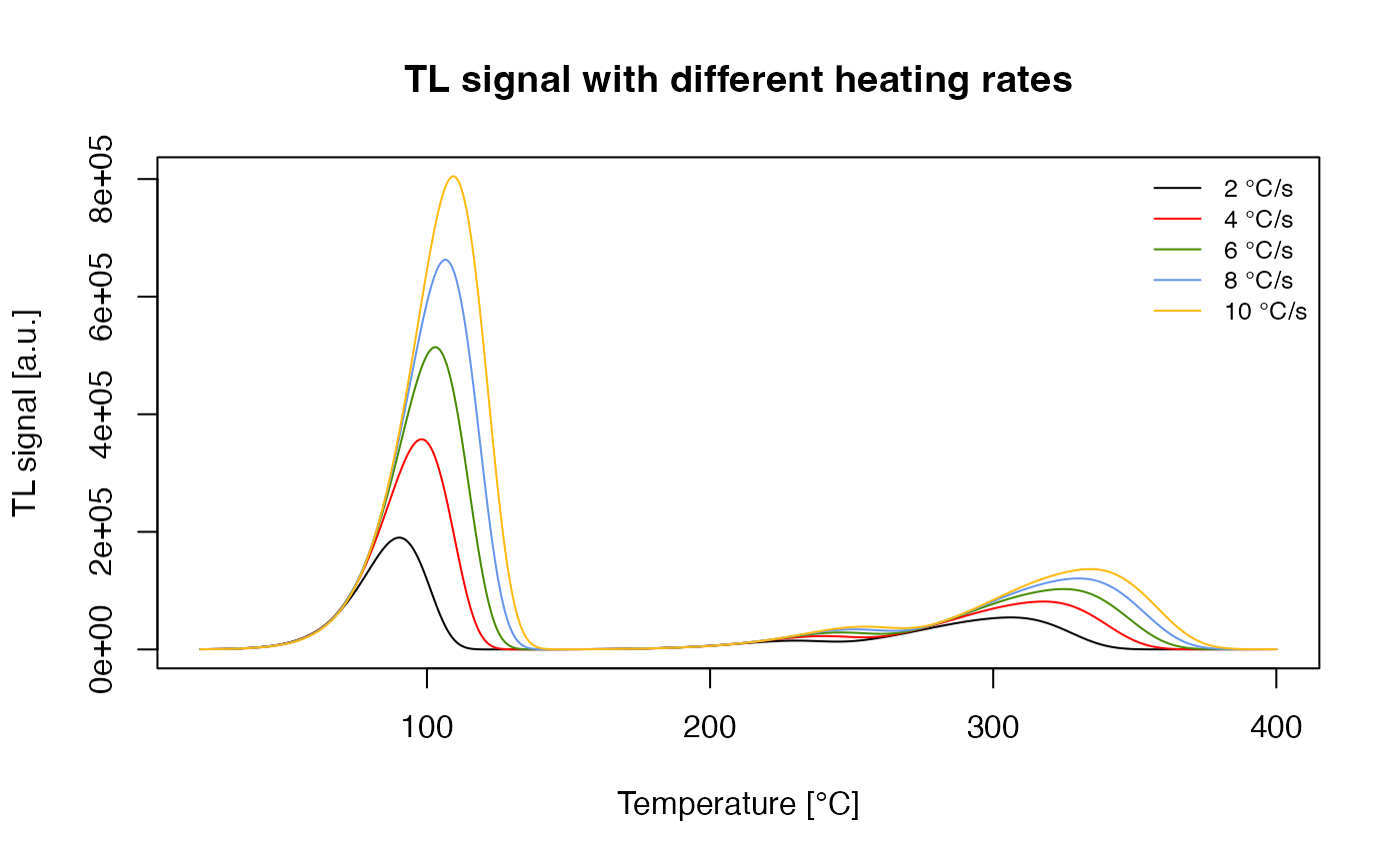
TL signal with different heating rates
Some notes to the code above:
- the return of the lapply function is a
RLum.Analysisobject, because of drop = FALSE -
recordType = TL$is necessary to match the character TL exact and not the concentrations -
merge_RLumis necessary to merge all the singleRLum.Analysisobjects in the list ‘model.output’ together to oneRLum.Analysisobject - to see the results with another parameter set, only
model = "..."has to be changed (see Sec. 2)
Simulating thermal activation characteristics (TACs)
Another frequently simulated phenomenon is the sensitisation of
quartz TL by \(\beta\)- or \(\gamma\)-irradiation followed by activation
at high temperatures Adamiec et al.
(2004), termed as thermal activation characteristics (TACs). For
a simulation sequence, the reader is referred to V. Pagonis et al. (2008a), Tab. 1. To simulate
this phenomenon with the model_LuminescenceSignals()
function, a loop causing a stepwise increase of the activation
temperature is needed. The resulting intensity of the 110 °C TL peak can
be plotted against the activation temperature, which shows TAC for the
model parameters of “Pagonis2007”.
##set temperature
act.temp <- seq(from = 80, to = 600, by = 20)

##loop over temperature
model.output <- vapply(X = act.temp, FUN = function(x) {

  ##set sequence, note: sequence includes sample history
  sequence <- list(
    IRR = c(20, 1, 1e-11),
    IRR = c(20, 10, 1),
    PH = c(x, 1),
    IRR = c(20, 0.1, 1),
    TL = c(20, 150, 5)
    )

  ##run simulation
  temp <- model_LuminescenceSignals(
    sequence = sequence,
    model = "Pagonis2007",
    simulate_sample_history = TRUE,
    plot = FALSE,
    verbose = FALSE
    )

  ## "TL$" for exact matching TL and not (TL)
  TL_curve <- Luminescence::get_RLum(temp, recordType = "TL$")

  ##return max value in TL curve
  return(max(get_RLum(TL_curve)[,2]))

}, FUN.VALUE = 1)
TAC with parameter set of ‘Pagonis2007’
Simulating dependency of the OSL signal on the illumination power density
The function model_LuminescenceSignals() is also capable
of simulating OSL phenomena. The next figure shows the dependency of the
OSL signal on the power density of illumination for the model
“Bailey2004”.
##set optical power [%]
optical_power <- c(0,20,40,60,80,100)

##loop over power
model.output <- lapply(optical_power, function(x){

  ##set sequence
  sequence <- list(
    IRR = c(20, 50, 1),
    PH = c(220, 10, 5),
    OSL = c(125, 50, x))


  data <-  model_LuminescenceSignals(
    sequence = sequence,
    model = "Bailey2004",
    plot = FALSE,
    verbose = FALSE)

  ##"OSL$" for exact matching OSL and not (OSL)
  return(Luminescence::get_RLum(data, recordType = "OSL$", drop = FALSE))

})

##merge output
model.output.merged <- Luminescence::merge_RLum(model.output)

##plot results
Luminescence::plot_RLum(
  object = model.output.merged,
  xlab = "Illumination time [s]",
  ylab = "OSL signal [a.u.]",
  legend.text = paste("Optical power ", 20 * optical_power / 100," mW/cm^2"),
  combine = TRUE
  )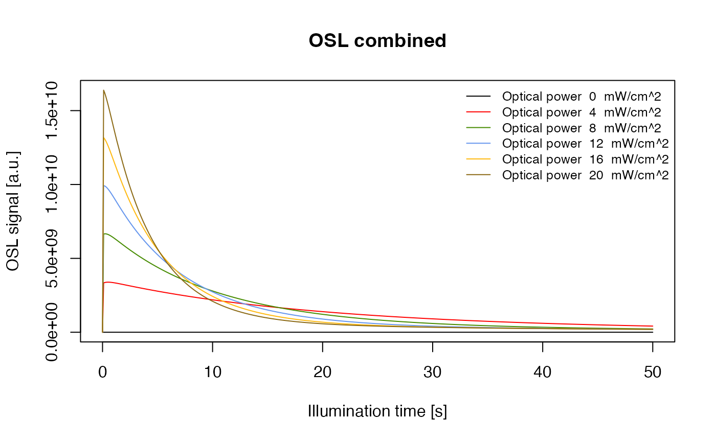
OSL measurement with different optical power densities with the parameter set of ‘Bailey2004’
Simulating and analysing SAR measurements
For simulating a DRT, it is necessary to define a sequence with the
keyword Irr_2recover, as mentioned in Section 4.3.
It should be mentioned that a simulation of a combinded PHPT and DRT may be very time-consuming, because for every preheat temperature a complete SAR cycle has to be run. A typical DRT sequence featuring various PH temperatures in ‘RLumModel’ is listed below. Note that in such a DRT simulation a loop over different preheat temperatures has to be written, utilising characteristic parameters from the literature. The test dose is set to 10% and the regeneration dose points to 40%, 70%, 130%, 160%, 0% and 40% of the recovery dose.
The data created by ‘RLumModel’ can be directly passed to the
functions Luminescence::analyse_SAR.CWOSL() and
Luminescence::plot_DRTResults() for routine analyses and
plotting.
##set PH temperatures
PH_temp <- seq(from = 160, to = 300, by = 20)

##set regeneration doses
RegDose = c(0, 80, 140, 260, 320, 0, 80)

##loop over PH temperatures
DRT.output <- lapply(PH_temp, function(x){

  sequence <- list(
       RegDose = RegDose,
       TestDose = 20,
       PH = x,
       CH = x,
       OSL_temp = 125,
       Irr_2recover = 200)

  model.output <- model_LuminescenceSignals(
       sequence = sequence,
       model = "Pagonis2008",
       plot = FALSE,
       verbose = FALSE)

  results <- Luminescence::analyse_SAR.CWOSL(
       object = model.output,
       signal.integral.min = 1,
       signal.integral.max = 7,
       background.integral.min = 301,
       background.integral.max = 401,
       fit.method = "EXP",
       dose.points = RegDose,
       plot = FALSE)

  temp <- get_RLum(results)
  out <- data.frame(
    De = temp$De,
    De.error = temp$De.Error)

  return(out)
})
## [plot_GrowthCurve()] Fit: EXP (interpolation) | De = 179.1 | D01 = 101.51
## [plot_GrowthCurve()] Fit: EXP (interpolation) | De = 179.46 | D01 = 101.46
## [plot_GrowthCurve()] Fit: EXP (interpolation) | De = 180.18 | D01 = 101.4
## [plot_GrowthCurve()] Fit: EXP (interpolation) | De = 180.6 | D01 = 101.41
## [plot_GrowthCurve()] Fit: EXP (interpolation) | De = 182.24 | D01 = 101.44
## [plot_GrowthCurve()] Fit: EXP (interpolation) | De = 179.85 | D01 = 102.26
## [plot_GrowthCurve()] Fit: EXP (interpolation) | De = 166.73 | D01 = 111.51
## [plot_GrowthCurve()] Fit: EXP (interpolation) | De = 159.15 | D01 = 161.2
##output as data.frame for plot_DRTResults
DRT.result <- as.data.frame(do.call(rbind, DRT.output))

##plot DRT.results
Luminescence::plot_DRTResults(
     DRT.result,
     preheat = PH_temp,
     given.dose = 200)
Dose recovery test (DRT) with the parameter set of ‘Pagonis2008’
In the code above, plot = FALSE was chosen, because a
single OSL plot is not necessary to analyse a SAR sequence. To calculate
a De from the produced RLum.Analysis object
‘model.output’, the function
Luminescence::analyse_SAR.CWOSL() is suitable. After
specifying a number of evaluation parameters (signal and background
integration interval, dose points and fit function for the dose response
curve) and the analysis process, the reduced data are stored in an
RLum.Results object, here termed ‘results’ . A background
integration interval from 301 to 401 translates to the signal from 30 s
to 40 s, because a channel has the default width of 0.1 s. Accordingly,
the signal integral ranges from 0.1 s to 0.7 s.
##set RegDose
RegDose = c(0, 80, 140, 260, 320, 0, 80)

##set sequence
sequence <- list(
  RegDose = RegDose,
  TestDose = 20,
  PH = 220,
  CH = 220,
  OSL_temp = 125
  )

##model
model.output <- model_LuminescenceSignals(
  sequence = sequence,
  model = "Pagonis2008",
  plot = FALSE,
  verbose = FALSE
  )

##analyse SAR sequence and plot only the resulting growth curve
results <- Luminescence::analyse_SAR.CWOSL(
  model.output,
  signal.integral.min = 1,
  signal.integral.max = 7,
  background.integral.min = 301,
  background.integral.max = 401,
  fit.method = "EXP",
  dose.points = RegDose,
  verbose = FALSE,
  plot.single = c(6)
  )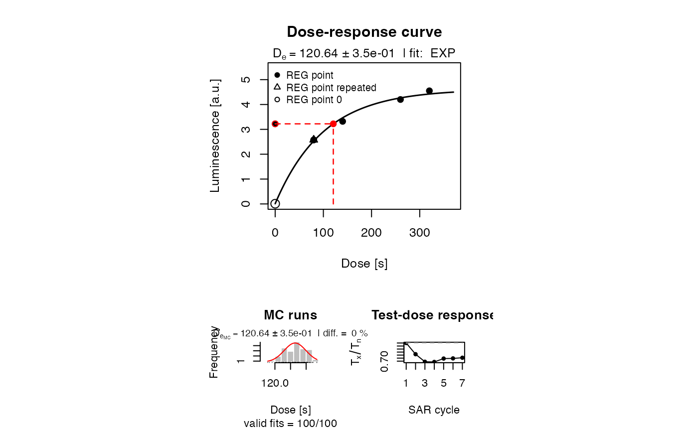
SAR protocol with the parameter set of ‘Pagonis2008’
Miscellaneous
Accessing applied modelling parameters
Sometimes it is useful to extract the used modelling parameters.
Since the output is an RLum.Analysis-object compatible with
the R package 'Luminescence', this can be achieved with the
following code lines (note: we have shorted the terminal output below
using the function head()):
## $parms.N1
## [1] 1.5e+07
##
## $parms.N2
## [1] 1e+07
##
## $parms.N3
## [1] 4e+07
##
## $parms.N4
## [1] 2.5e+08
##
## $parms.N5
## [1] 5e+10
##
## $parms.N6
## [1] 5e+09
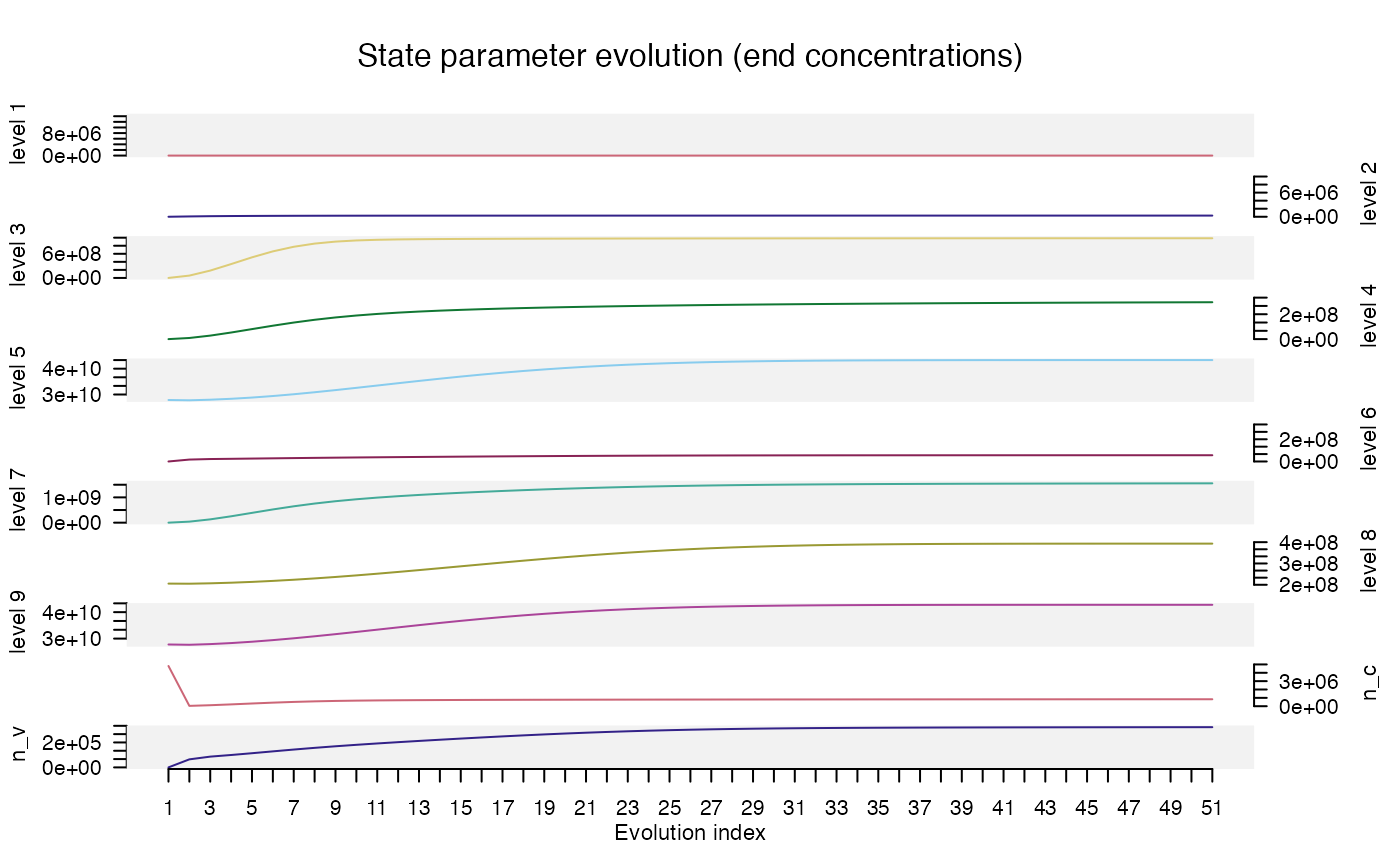
Trace parameter state evolution
An exciting feature of 'RLumModel' is that it allows you
to gain insight into the evolution of different parameter states beyond
a single simulation, which would show you how numerical parameters
change if the solver runs over the equations. For instance, assume you
have a sequence of different stimulation steps (TL, OSL etc.). You want
to know how the system, for which the solver has to find a solution,
changes from one sequence step to another. This is of interest because
the initial state of the system of each step will determine the shape of
the curve. Let’s think of the following sequence that, after an initial
TL readout, adds a dose followed by a TL measurement, then another
irradiation, another TL measurement and so on.
dose_points <- seq(8,600, length.out = 50)
sequence <- c(
  list(TL = c(20 , 500 , 2)),
  unlist(lapply(dose_points, function(d){
    list(
      IRR = c(20 , d , 0.03),
      TL = c(20 , 250, 2))

  }), recursive = FALSE))
This sequence can modelled as shown above, here we use again the
Baily2001 model:
results <- model_LuminescenceSignals(
  model = "Bailey2001",
  sequence = sequence,
  plot = FALSE,
  show_structure = FALSE,
  simulate_sample_history = FALSE,
  verbose = FALSE)
What we did already above was to show the resulting TL curves, and we do this again, just to see how they look like.
Luminescence::plot_RLum(
  get_RLum(results, recordType = "^TL$", drop = FALSE),
  combine = TRUE,
  xlim = c(20,120),
  records_max = 10,
  legend.pos = "topleft",
  plot.single = TRUE)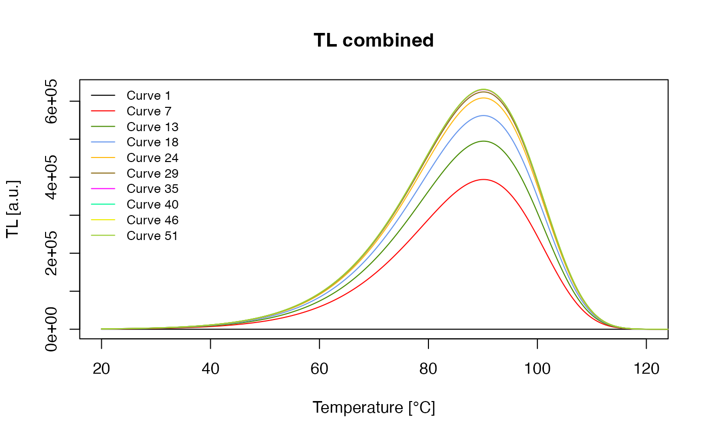
Now we go one step further and focus our interest on the evolution of
each parameter set at the end of each sequence step. Extracting all the
data manually is possible, but a little cumbersome, so instead, we will
use the function trace_StateParameterEvoluation() (this
function was introduced with 'RLumModel' v0.2.10).
trace_ParameterStateEvolution(results)