RLumModel - Using own parameter sets

Johannes Friedrich, University of Bayreuth

2022-02-20

Introduction

With ‘RLumModel’ ≥ 0.2.0 is it possible to simulate quartz luminescence behaviour of own parameters or parameter sets, which are not included in the package but also known in literature. Widely used OTOR (One-Trap-One-Recombination-center) models can be included, too. This vignette gives three comprehensive examples how to implement parameter sets and proves the results recalculating the original simulations.

‘RLumModel’ offers maximum flexibility and fast calculation of ordinary first-order differential equations (ODEs) describing luminescence behaviour, because of:

• flexible handling of different numbers of electron traps and hole centres in generating the model equations. The user has not to care about coding ODEs in R.
• Solving these equations is performed with C++ (Eddelbuettel 2013) and offers a fast calculation.

Examples

This chapter shows the handling of own parameter sets with ‘RLumModel’. For this purpose three model parameters known from literature were taken: Pagonis et al. (2009), Lawless, Chen, and Pagonis (2009) and Chen and Pagonis (2013).

Pagonis 2009

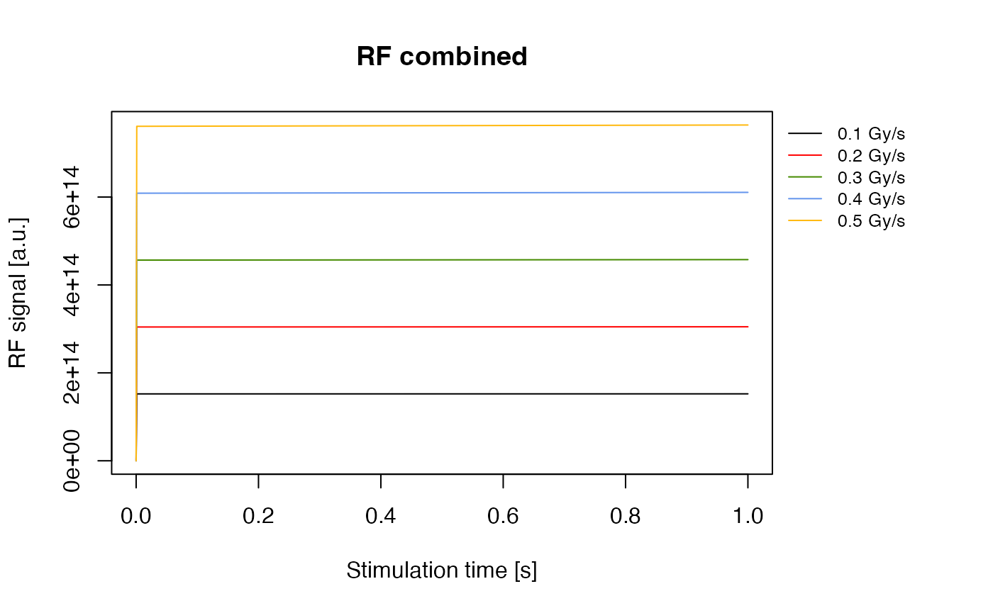
Pagonis et al. (2009) presented parameters for their luminescence modelling of radioluminescence. This model was built for Al₂O₃, but the rate equations are identical with describing electron movements in quartz. Below is a step-by-step manual for involving these parameters in ‘RLumModel’ and re-calculating the simulationa made by Pagonis et al. (2009). Note that in the original publication Figure 3 and Figure 6 are inconsistent with each other. For a doserate of 0.1 Gy/s an initial RL intensity of ca. 1.5e14 is obtained (see Figure 6 in original publication and simulations below).

Set parameters

First of all the model parameters had to be set. In ‘RLumModel’ this can be done via . The list has to contain the following items:

• N: Concentration of electron- and hole traps [cm^-3]
• E: Electron/Hole trap depth [eV]
• s: Frequency factor [s^-1]
• A: Conduction band to electron trap and valence band to hole trap transition probability [s^-1 cm ³].
• B: Conduction band to hole centre transition probability [s^-1 cm ³].
• Th: Photo-eviction constant or photoionisation cross section, respectively. If not set: by default 0.
• E_th: Thermal assistence energy [eV]. If not set: by default 0.
• k_B: Boltzman constant 8.617e-05 [eV/K]. If not set: by default 8.617e-05.
• W: activation energy 0.64 [eV] (for UV). If not set: by default 0.64.
• K: 2.8e7 (dimensionless constant). If not set: by default 2.8e7.
• model: “customized”
• R (optional): Ionisation rate (pair production rate) equivalent to 1 Gy/s [s^-1 cm ^-3]

Note:

• Not every publication uses the same definition of parameter A and B.
• When no thermal quenching is expected, set K = 0. A numerical value of W is necessary, if .
• The parameter model = "customized" is necessary to not load a stored model within the RLumModel pacakge.
• The luminescence center, which is responsible for the luminescence production (TL-, OSL-, RF-signal), has to be the last entry in the model parameters, see examples below.
• For further details of the parameter see Bailey (2001) and Wintle (1975).
• The first two entries in N, A and B belong to the electron traps and the last two entries to the hole centres. This order is necessary.
• The first entry in N, E, s, A, B, Th and E_th belong to the first energy level (e.g. 110°C), the second, third, … entries to second, third, … energy levels.
• The entries Th and E_th are not necessary, because when they miss in the definition of the own parameters they will automatically be set to 0.

own_parameters <- list(
  N = c(2e15, 2e15, 2.4e16, 1e17),
  E = c(0, 0, 0, 0),
  s = c(0, 0, 0, 0),
  A = c(2e-8, 2e-9, 4e-9, 1e-8),
  B = c(0, 0, 5e-11, 4e-8),
  K = 0,
  model = "customized",
  R = 1.7e15)

It is important to notice, that in Pagonis et al. (2009) B is the valence band to hole centre probability, but in Bailey (2001) this is A_j. The default setting of RLumModel is the definition by Bailey (2001) and so the values of B (in Pagonis et al. (2009)) are A in the notation above.

As a next step it is possible to set own starting-parameters, also called state parameters. In the case of Pagonis et al. (2009) they submitted initial concentrations of electrons and holes. This can be done via:

own_state_parameters <- c(0, 0, 0, 9.4e15)

Here the first entry is the first electron trap, the second entry the second electron trap, the third entry the hole center and the fourth entry the luminescence center responsible for the RF signal. The vector own_state_parameters needs as much entries as energy levels used in the model.

Running the simulation with RLumModel

When all parameters are set, the simulation can be started. The main function in RLumModel is model_LuminescenceSignals() and the usage with own parameter sets is described below. For a general overview for creating a sequence, running RLumModel with stored models etc. the user is referred to Friedrich, Kreutzer, and Schmidt (2016) and to the vignette RLumModel - Getting started with RLumModel.

For simulating the results of Pagonis et al. (2009) the follwing sequence is needed.

sequence <- list(RF = c(20, 0.1, 0.1))

This sequence describes a radiofluorescence simulation at 20 °C with a dose of 0.1 Gy and a dose rate of 0.1 Gy/s, so the stimulation time is 1s.

The parameters own_parameters and own_state_parameters in model_LuminescenceSignals() are prepared for using own created parameter sets. Parameter model = "customized" is necessary to not load stored parameters.

RF_Pagonis2009 <- model_LuminescenceSignals(
  model = "customized", 
  sequence = sequence, 
  own_parameters = own_parameters, 
  own_state_parameters = own_state_parameters,
  verbose = FALSE)

RF signal for 0.1 Gy/s

As in the original publication, initially the RF signal increases and is followed by an approximately linear region until the stimulation ends. Figure 5 in Pagonis et al. (2009) shows the concentration of the luminescence center m1 for the stimulation time of 1s. With RLumModel this can be plotted very fast with the following command (for a detailed description see vignette RLumModel - Getting started with RLumModel

concentration_m1 <- Luminescence::get_RLum(
  RF_Pagonis2009,
  recordType = c("conc. level 4"))
  
Luminescence::plot_RLum(
  concentration_m1, 
  ylim = c(9.2e15, 9.6e15))

Concentration of m1 during RF

Re-calculate the original results

Reproducing Figure 3 and Figure 6 in Pagonis et al. (2009) a loop over different dose rates is necessary. The following code lines are able to run the model for five different dose rates from 0.1 to 0.5 Gy/s and plot all contained RF curves and the initial RF signal. For a more detailed descripton of the loop and the single commands therein the user is referred to Friedrich, Kreutzer, and Schmidt (2016) and the vignette RLumModel - Getting started with RLumModel.

dose.rate <- seq(from = 0.1, to = 0.5, by = 0.1)

model.output <- lapply(dose.rate, function(x) {
    
    sequence <- list(RF = c(20, x, x))
    
    RF_data <- model_LuminescenceSignals(
      model = "customized", 
      sequence = sequence, 
      own_parameters = own_parameters, 
      own_state_parameters = own_state_parameters,
      verbose = FALSE,
      plot = FALSE
    )
    
    ## "RF$" for exact matching RF and not (RF)
    return(get_RLum(RF_data, recordType = "RF$", drop = FALSE))
    
  })

model.output.merged <- merge_RLum(model.output)

plot_RLum(
 object = model.output.merged,
 xlab = "Stimulation time [s]",
 ylab = "RF signal [a.u.]",
 legend.text = paste(dose.rate, "Gy/s"),
 legend.pos = "outside",
 combine = TRUE)

RF signals for different dose rates

The following code calcultes the initial RF signal for the five different dose rates.

dose.rate <- seq(from = 0.1, to = 0.5, by = 0.1)

model.output <- vapply(X = dose.rate, FUN = function(x) {
    
    sequence <- list(RF = c(20, x, x))
    
    temp <- model_LuminescenceSignals(
      model = "customized", 
      sequence = sequence, 
      own_parameters = own_parameters, 
      own_state_parameters = own_state_parameters,
      verbose = FALSE,
      plot = FALSE
    )
    
    ## "RF$" for exact matching RF and not (RF)
    RF_curve <- get_RLum(temp, recordType = "RF$")
    
    return(max(get_RLum(RF_curve)[2,2]))
    
  }, FUN.VALUE = 1)

Initial RF signal for different dose rates with parameters of Lawless 2009

The results show that ‘RLumModel’ is able to simulate the same results as published in Pagonis et al. (2009) with only little effort. All these examples can be modified to own needs, e.g. own sequences or own parameters.

Lawless 2009

Lawless, Chen, and Pagonis (2009) investigateted the sublinear dose dependence of TL and OSL. They published a set of model parameters to simulate the behaviour of the quartz luminescence system during different dose rates. In contrast to the example above, this simulation has no state parameters and so they were not definded.

Set parameters and recalculate the results

All used parameters are defined in the named list own_parameters. K=0 was chosen, because no thermal quenching was simulated. Note: In the “Bailey 2001” notation B has the same meaning as Am in Lawless, Chen, and Pagonis (2009) (for details see example in chapter 2.1.1).

own_parameters <- list(
  N = c(1e14, 1e15),
  E = c(0, 0),
  s = c(0, 0),
  A = c(1e-13, 1e-14),
  B = c(0, 1e-7),
  K = 0,
  model = "customized",
  R = 1e8)

sequence <- list(RF = c(20, 100, 1))

RF_Lawless_2009 <- model_LuminescenceSignals(
  model = "customized", 
  sequence = sequence, 
  own_parameters = own_parameters,
  verbose = FALSE,
  plot = FALSE)

concentration_n <- Luminescence::get_RLum(
  RF_Lawless_2009, 
    recordType = c("conc. level 1"))

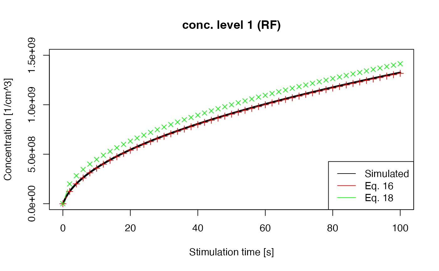
This code leads to the following results and shows the same as plotted in Lawless, Chen, and Pagonis (2009), Fig. 2 (plot commands not shown here). More details to the equations mentioned in the legend are available in the original publication.

Concentration of Level 1 with numerical and analytical solutions

Chen 2013

Chen and Pagonis (2013) published a numerical model to investigate the quasi-equilibrium assumptions in TL. For the description of the system a OTOR model was used.

Set parameters

This model is the first in this vignette which did not start its simulation at 20 °C. For this cases, model_LuminescenceSignals() offers a parameter called own_start_temperature. This parameter offers maximal flexibility for the user to set the initial temperature of the simulation. The parameter takes effect when model = "customized" is used, see example below.

own_parameters <- list(
  N = c(1e9, 0),
  E = c(0.4, 0),
  s = c(1e11, 0),
  A = c(1e-9,0),
  B = c(0, 1e-10),
  K = 0,
  model = "customized")

own_state_parameters <- c(1e8, 1e8)

own_start_temperature <- -220

sequence <- list(TL = c(-220, 130, 1))

Re-calculate the original results

Here the parameter own_start_temperature from the function model_LuminescenceSignals() is used to set the beginning of the measurement to -220°C. It is important, that ‘RLumModel’ always uses temperatures in °C.

TL_Chen2013 <- model_LuminescenceSignals(
  model = "customized", 
  sequence = sequence, 
  own_parameters = own_parameters, 
  own_state_parameters = own_state_parameters,
  own_start_temperature = own_start_temperature,
  verbose = FALSE)

TL with parameter sets of Chen 2013

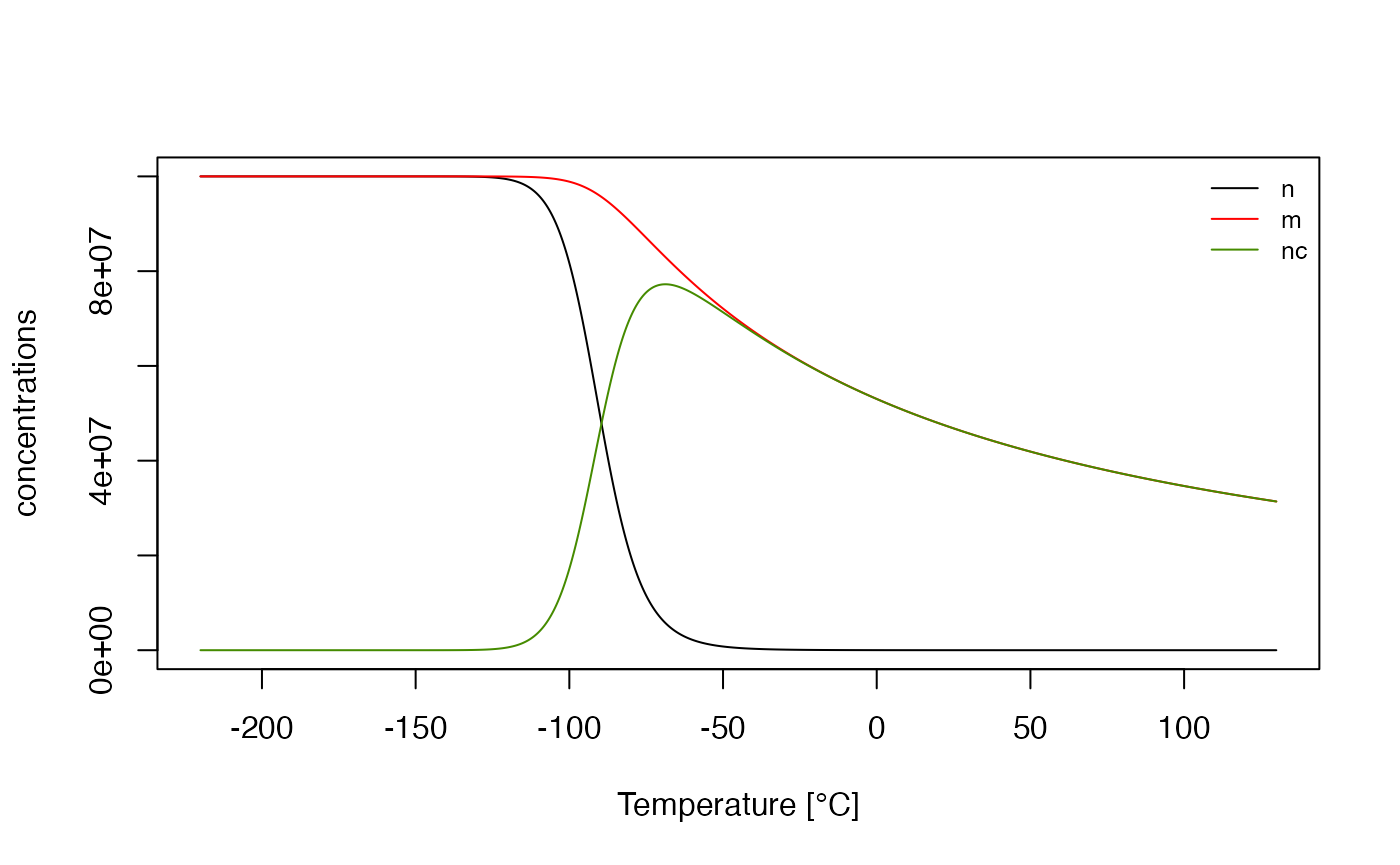
With this result it is possible to plot the concentration of every single energy level, leading to the following plot (see also Fig. 6 in Chen and Pagonis (2013))

Concentrations of different energy levels

Summary

This vignette showed the potential of the R package ‘RLumModel’ to use own parameter sets simulating quartz luminescence behaviour. Quartz as well as Al₂O₃ luminescence phenomena can be numerically described and graphically plotted.

References

Bailey, R M. 2001. “Towards a General Kinetic Model for Optically and Thermally Stimulated Luminescence of Quartz.” Radiation Measurements 33: 17–45.

Chen, R, and V Pagonis. 2013. “On the quasi-equilibrium assumptions in the theory of thermoluminescence (TL).” Journal of Luminescence 143: 734–40.

Eddelbuettel, Dirk. 2013. Seamless R and C++ integration with Rcpp. Springer.

Friedrich, Johannes, Sebastian Kreutzer, and Christoph Schmidt. 2016. “Solving ordinary differential equations to understand luminescence: ’RLumModel’, an advanced research tool for simulating luminescence in quartz using R .” Quaternary Geochronology 35: 88–100.

Lawless, J L, R Chen, and V Pagonis. 2009. “Sublinear Dose Dependence of Thermoluminescence and Optically Stimulated Luminescence Prior to the Approach to Saturation Level.” Radiation Measurements 44 (5): 606–10.

Pagonis, V, J L Lawless, R Chen, and C Andersen. 2009. “Radioluminescence in Al\({_2}\)O\({_3}\):C – Analytical and Numerical Simulation Results.” Journal of Physics D: Applied Physics 42 (17): 175107.

Wintle, AG. 1975. “Thermal Quenching of Thermoluminescence in Quartz.” Geophysical Journal International 41 (1): 107–13.