RLumModel - Simulating luminescence in Al2O3
Johannes Friedrich, University of Bayreuth
2022-02-20
Source:vignettes/RLumModel_-_Simulating_luminescence_in_Al2O3.Rmd
RLumModel_-_Simulating_luminescence_in_Al2O3.RmdIntroduction
This vignette describes the usage of the R-package
‘RLumModel’ for simulating Al2O3 behaviour. In
literature a lot of parameters for describing the thermoluminescence
(TL) and/or optical stimulated luminescence (OSL) are given. We give
same examples for simulating different phenomena of luminescence in
Al2O3. Note that most of the model do not support
TL and OSL simulations. So please be careful when
creating sequences. The models presented in Sec. 2.1 and 2.2 support TL
simulations, but no OSL because parameters for E_th
(Thermal assistance energy) and Th (Photo-eviction constant
or photoionisation cross section).
Examples
All examples need the R package RLumModel, so let’s load it!
Akselrod 1998
Akselrod et al. (1998) presented parameters for modelling the effect of quenching TL signals. This model was built for Al2O3, but the rate equations are identical with describing electron movements in quartz. Below is a step-by-step introduction for involving these parameters in ‘RLumModel’ and re-calculating the simulationa from Figure 9 in Akselrod et al. (1998).
Set own starting parameters
For a detailed introduction to own parameter sets in RLumModel, see vignette RLumModel - Using own parameter sets.
As a next step it is possible to set own starting-parameters, also called state parameters. In the case of Akselrod et al. (1998) they submitted initial concentrations of electrons and holes. This can be done via:
own_state_parameters <- c(0, 0, 1e11)Here the first entry is the first electron trap, the second entry the
second electron trap and the third entry the luminescence centre
responsible for the TL signal. The vector
own_state_parameters needs as much entries as energy levels
used in the model.
Calculate thermal quenching effect
The effect of quenching luminescence signals will be simulated. In
RLumModel it is possible to submit the parameter K as an
indicator for recognising thermal quenching or not. If the parameter is
set to 0 thermal quenching will be neglected. Otherwise it
wil be calculated.
W <- c(0, 1.05)

TL_Akselrod_1998 <- lapply(W, function(W){

  own_parameters <- list(
    N = c(1e18, 1e17, 1e18),
    E = c(1.25, 0, 0),
    s = c(1e13, 0, 0),
    A = c(1e-16, 1e-16, 2e-17),
    B = c(0, 0, 1e-16),
    K = ifelse(W == 0, 0, 1e12),
    W = W,
    model = "customized",
    R = 1e13)

  sequence <- list(
    IRR = c(20, 0.225, 0.01),
    TL = c(20, 300, 1))

  model_output <- model_LuminescenceSignals(
    model = "customized",
    sequence = sequence,
    own_parameters = own_parameters,
    own_state_parameters = own_state_parameters,
    verbose = FALSE,
    plot = FALSE)

  return(get_RLum(model_output, recordType = "TL$", drop = FALSE))
})

merge_results <- merge_RLum.Analysis(TL_Akselrod_1998)

plot_RLum.Analysis(
  merge_results,
  legend.text = c("Unquenched", "Quenched"),
  combine = T)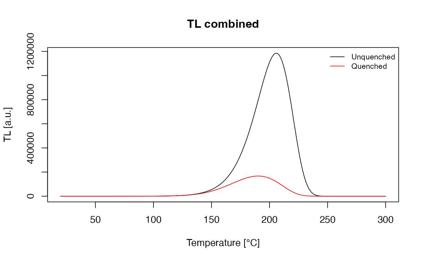
The effect of thermal quenching for TL signals
Pagonis 2007
Pagonis, Chen, and Lawless (2007) published three different parameter sets for Al2O3 chips. Here we analyse ‘Chip101’ and show how to re-calculate the results presented in the publication.
Caclualte TL signal dependend on the given dose
We now have to define the sequence for simulating the TL behaviour.
For that purpose different doses are given before the TL measurement. To
handle this a lapply command was used. The result is the
combined plot of all simulated TL measurements.
dose <- 10^seq(-1, 3.5, 0.5)

Pagonis_2007 <- lapply(dose, function(dose){

  sequence <- list(
    IRR = c(20, dose, 1),
    PAUSE = c(20, 60),
    TL = c(20, 250, 1))

  model_output <- model_LuminescenceSignals(
    model = "customized",
    sequence = sequence,
    own_parameters = own_parameters,
    own_state_parameters = own_state_parameters,
    verbose = FALSE,
    plot = FALSE)

  return(Luminescence::get_RLum(model_output, recordType = "TL", drop = FALSE))
})

merge_results <- Luminescence::merge_RLum.Analysis(Pagonis_2007)

Luminescence::plot_RLum.Analysis(
  merge_results,
  subset =  list(recordType = "TL$"),
  xlim = c(100, 250),
  legend.text = paste0(round(dose, digits = 2), " Gy"),
  combine = T)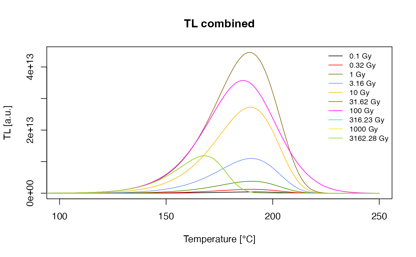
TL signal for different given doses
Calculate maximum TL signal and concentration of L-centre
Figure 2 in the original publiction by Pagonis, Chen, and Lawless (2007) will be plotted with the following commands. The following code commands are able to calculate the maximum of the TL signal of all curves.
TL_max <- vapply(1:length(Pagonis_2007), function(x){

  TL <- get_RLum(get_RLum(Pagonis_2007[[x]], recordType = "TL$"))

  return(max(TL[,2]))

}, FUN.VALUE = 1)
Now the calculation of the concentration:
m1_max <- vapply(1:length(Pagonis_2007), function(x){

  m1 <- get_RLum(get_RLum(Pagonis_2007[[x]], recordType = "conc. level 4"))

  return(m1[1,2])

}, FUN.VALUE = 1)
When plotting L-centre concentration vs. dose or TLmax vs. dose the same results as presented in Fig. 2 in Pagonis, Chen, and Lawless (2007) are reached.
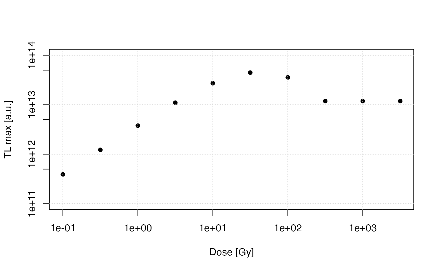
TL max vs. dose
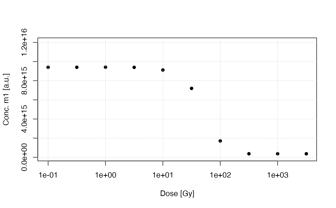
Concentration of m1 (L-centre) vs. dose
Concentration at the end of irradiation
dose <- seq(1,400, 1)

Fig_5 <- lapply(dose, function(dose){

  sequence <- list(
    RF = c(20, dose, 1))

  model_output <- model_LuminescenceSignals(
    model = "customized",
    sequence = sequence,
    own_parameters = own_parameters,
    own_state_parameters = own_state_parameters,
    verbose = FALSE,
    plot = FALSE)

})
n1 <- vapply(1:length(Fig_5), function(x){

  temp <- get_RLum(get_RLum(Fig_5[[x]], recordType = "conc. level 1"))

  return(temp[nrow(temp),2])

}, FUN.VALUE = 1)

n2 <- vapply(1:length(Fig_5), function(x){

  temp <- get_RLum(get_RLum(Fig_5[[x]], recordType = "conc. level 2"))

  return(temp[nrow(temp),2])

}, FUN.VALUE = 1)

m1 <- vapply(1:length(Fig_5), function(x){

  temp <- get_RLum(get_RLum(Fig_5[[x]], recordType = "conc. level 4"))

  return(temp[nrow(temp),2])

}, FUN.VALUE = 1)

m2 <- vapply(1:length(Fig_5), function(x){

  temp <- get_RLum(get_RLum(Fig_5[[x]], recordType = "conc. level 3"))

  return(temp[nrow(temp),2])

}, FUN.VALUE = 1)
plot(dose, m2, type = "l", ylim = c(0, 1.5e16), xlim = c(0, 500), xlab= "Dose [Gy]", ylab = "Concentration [a.u.]")
lines(dose, n2, col = "red")
lines(dose, m1, col = "green")
lines(dose, n1, col = "blue")

legend("topright", legend = c("n1", "n2", "m1", "m2"), col = c("blue", "red", "green", "black"), lwd = 1, bty = "n")
grid()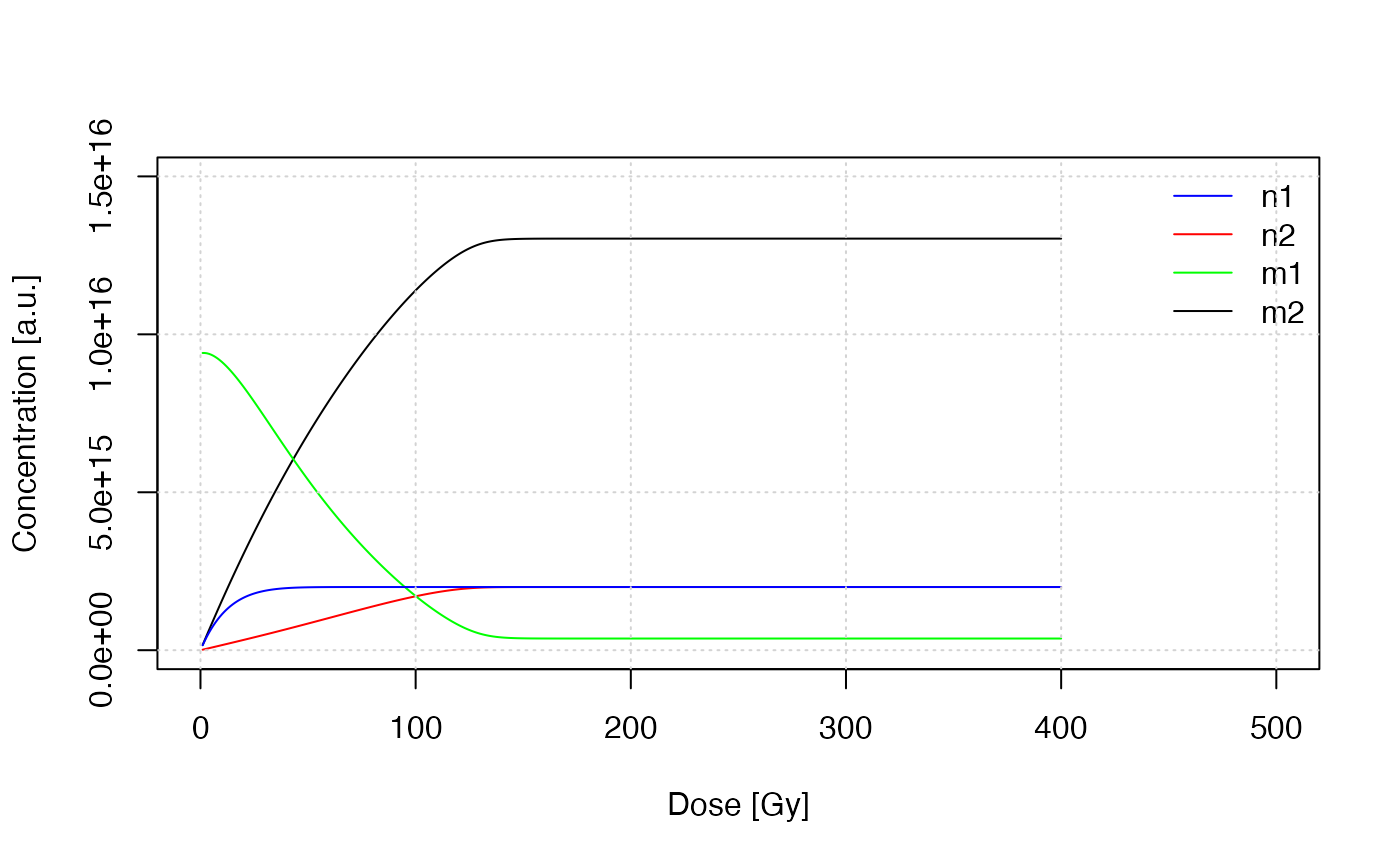
Concentration in different traps at the end of the irradiation
Summary
This vignette showed the potential of the R package ‘RLumModel’ to simulate Al2O3 behaviour. Two different models known from literature were re-compiled in the framework of RLumModel.