Apply the Huntley (2006) model — calc_Huntley2006 • Luminescence

The function calculates the expected sample specific fraction of saturation based on the model of Huntley (2006), using the approach as implemented in Kars et al. (2008) or Guralnik et al. (2015).

Usage

calc_Huntley2006(
  data,
  LnTn = NULL,
  rhop,
  ddot,
  readerDdot,
  normalise = TRUE,
  fit.method = c("EXP", "GOK"),
  lower.bounds = c(-Inf, -Inf, -Inf, -Inf),
  cores = 1,
  summary = TRUE,
  plot = TRUE,
  ...
)

Arguments

data

data.frame (required): A data.frame with one of the following structures:

three columns with numeric values for dose (s), LxTx and LxTx error, in this order.
two columns with numeric values for dose (s) and LxTx, in this order. This assumes that errors on LxTx are missing, and a third column will be automatically attached with an arbitrary 5 % error on the provided LxTx values.
wide table, i.e. a data.frame with a number of columns divisible by 3 and where each triplet has the aforementioned column structure.

                        (optional)
     | dose (s)| LxTx | LxTx error |
     |  [ ,1]  | [ ,2]|    [ ,3]   |
     |---------|------|------------|
[1, ]|  0      | LnTn | LnTn error | (optional, see arg 'LnTn')
[2, ]|  R1     | L1T1 | L1T1 error |
 ... |    ...  |  ... |     ...    |
[x, ]|  Rx     | LxTx | LxTx error |

NOTE: The function assumes the first row of the data to be the Ln/Tn-value. If you want to provide more than one Ln/Tn-values, consider using argument LnTn.

LnTn

data.frame (optional): A two column data frame with the following structure:

     |  LnTn  |  LnTn error  |
     |  [ ,1] |      [ ,2]   |
     |--------|--------------|
[1, ]| LnTn_1 | LnTn_1 error |
[2, ]| LnTn_2 | LnTn_2 error |
 ... |   ...  |      ...     |
[x, ]| LnTn_x | LnTn_x error |

The function will calculate a mean Ln/Tn-value and uses either the standard deviation or the highest individual error, whichever is larger. If another mean value (e.g. a weighted mean or median) or error is preferred, this value must be calculated beforehand and used in the first row in the data frame for argument data.

NOTE: This argument should only be used to provide more than one Ln/Tn-value. If you provide LnTn-values with this argument, the data frame for the data-argument must not contain any LnTn-values.

rhop

numeric (required): A vector of length 2 for the density of recombination centres ($\rho$') and its error (see Huntley 2006). Note that $\rho$' must not be provided as the common logarithm. Example: rhop = c(2.92e-06, 4.93e-07).

ddot

numeric (required): A vector of length 2 for the environmental dose rate and its error. Expected unit: Gy/ka. Example: ddot = c(3.7, 0.4).

readerDdot

numeric (required): A vector of length 2 for the dose rate of the irradiation source of the OSL reader and its error. Expected unit: Gy/s. Example: readerDdot = c(0.08, 0.01).

normalise

logical (with default): If TRUE (the default) all measured and computed $\frac{L_x}{T_x}$ values are normalised by the pre-exponential factor A (see details).

fit.method

character (with default): Fit function of the dose response curve. Can either be "EXP" (default) or "GOK". Note that "EXP" (single saturating exponential) is the original function the model after Huntley (2006) and Kars et al. (2008) was designed to use. The use of a general-order kinetics function ("GOK") is an experimental adaptation of the model and should be used with great care.

lower.bounds

numeric (with default): A vector of length 4 for the values of the lower bounds to be applied when fitting the models with minpack.lm::nlsLM. In most cases, the default values (c(-Inf, -Inf, -Inf, -Inf)) are appropriate for finding a best fit, but sometimes it may be useful to restrict the lower bounds to e.g. c(0, 0, 0, 0). The values of the vectors are, respectively, for parameters a, D0, c and d in that order (parameter d is ignored when fit.method = "EXP"). More details can be found in fit_DoseResponseCurve.

cores

integer (with default): The number of cores to use. This will be capped to the number of available cores if set to too high.

summary

logical (with default): If TRUE (the default) various parameters provided by the user and calculated by the model are added as text on the right-hand side of the plot.

plot

logical (with default): enable/disable the plot output.

...

Further parameters:

verbose logical: Enable/disable output to the terminal (default = TRUE)
n.MC numeric: Number of Monte Carlo iterations (default = 10000)
cex numeric: Scaling of the plot (default = 1)
maxiter numeric: Number of iteration limits for nls fitting
trace logical: Enable/disable value tracing the terminal during fitting Note that it is generally advised to have a large number of Monte Carlo iterations for the results to converge. Decreasing the number of iterations will often result in unstable estimates.

All other arguments are passed to plot and fit_DoseResponseCurve (in particular mode for the De calculation mode, fit.force_through_origin, and fit.bounds).

Value

An RLum.Results object is returned:

Slot: @data

OBJECT	TYPE	COMMENT
`results`	data.frame	results of the of Kars et al. 2008 model
`data`	data.frame	original input data
`Ln`	numeric	Ln and its error
`LxTx_tables`	`list`	A `list` of `data.frames` containing data on dose, LxTx and LxTx error for each of the dose response curves. Note that these do not contain the natural `Ln` signal, which is provided separately.
`fits`	`list`	A `list` of `nls` objects produced by minpack.lm::nlsLM when fitting the dose response curves

Slot: @info

OBJECT	TYPE	COMMENT
`call`	`call`	the original function call
`args`	`list`	arguments of the original function call

Details

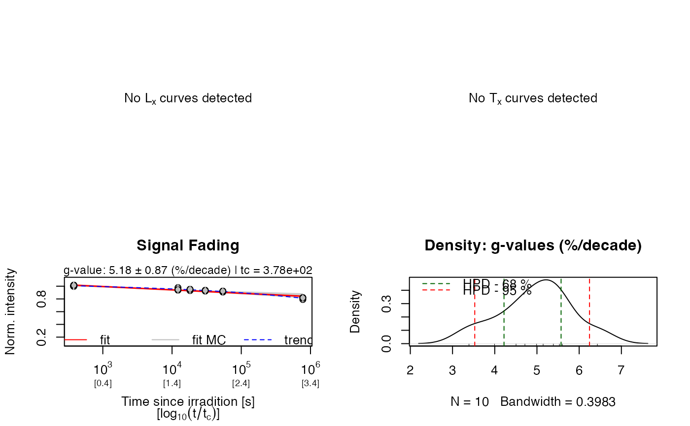
This function applies the approach described in Kars et al. (2008) or Guralnik et al. (2015), which are both developed from the model of Huntley (2006), to calculate the expected sample specific fraction of saturation of a feldspar and also to calculate fading corrected age using this model. $\rho$' (rhop), the density of recombination centres, is a crucial parameter of this model and must be determined separately from a fading measurement. The function analyse_FadingMeasurement can be used to calculate the sample specific $\rho$' value.

Kars et al. (2008) – Single saturating exponential

To apply the approach after Kars et al. (2008), use fit.method = "EXP".

Firstly, the unfaded $D_0$ value is determined through applying equation 5 of Kars et al. (2008) to the measured $\frac{L_x}{T_x}$ data as a function of irradiation time, and fitting the data with a single saturating exponential of the form:

$$\frac{L_x}{T_x}(t^*) = A \phi(t^*) \{1 - \exp(-\frac{t^*}{D_0}))\}$$

where

$$\phi(t^*) = \exp(-\rho' \ln(1.8 \tilde{s} t^*)^3)$$

after King et al. (2016) where $A$ is a pre-exponential factor, $t^*$ (s) is the irradiation time, starting at the mid-point of irradiation (Auclair et al. 2003) and $\tilde{s}$ ($3\times10^{15}$ s$^{-1}$) is the athermal frequency factor after Huntley (2006).

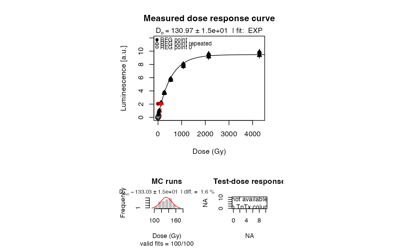
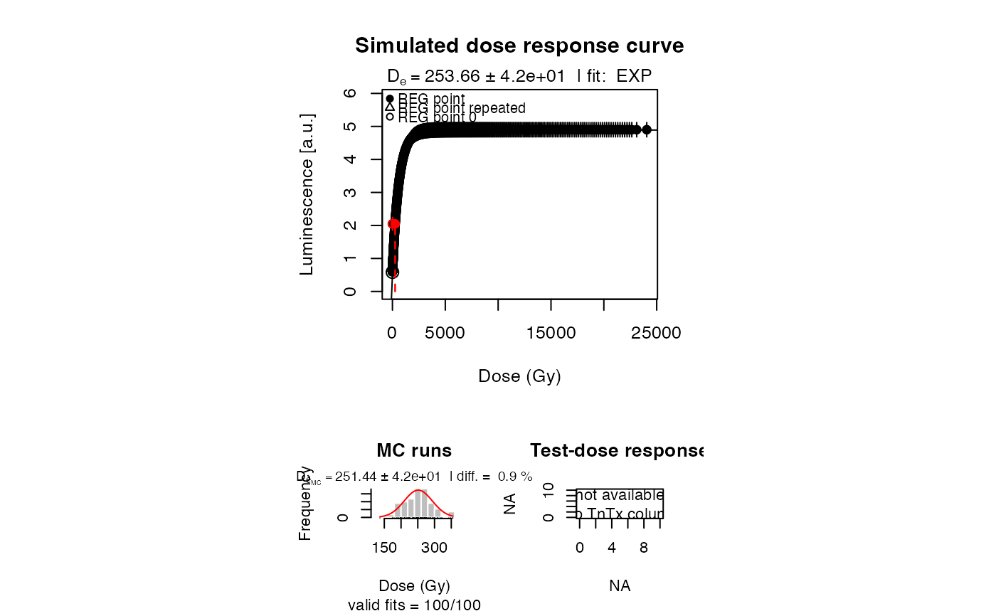
Using fit parameters $A$ and $D_0$, the function then computes a natural dose response curve using the environmental dose rate, $\dot{D}$ (Gy/s) and equations [1] and [2]. Computed $\frac{L_x}{T_x}$ values are then fitted using the fit_DoseResponseCurve function and the laboratory measured LnTn can then be interpolated onto this curve to determine the fading corrected $D_e$ value, from which the fading corrected age is calculated.

Guralnik et al. (2015) – General-order kinetics

To apply the approach after Guralnik et al. (2015) use fit.method = "GOK".

The approach of Guralnik et al. (2015) is very similar to that of Kars et al. (2008) but, instead of using a single saturating exponential, the model fits a general-order kinetics function of the form:

$$\frac{L_x}{T_x}(t^*) = A \phi (t^*)(1 - (1 + (\frac{1}{D_0}) t^* c)^{-1/c})$$

where $A$, $\phi$, $t^*$ and $D_0$ are the same as above and $c$ is a dimensionless kinetic order modifier (cf. equation 10 in Guralnik et al., 2015).

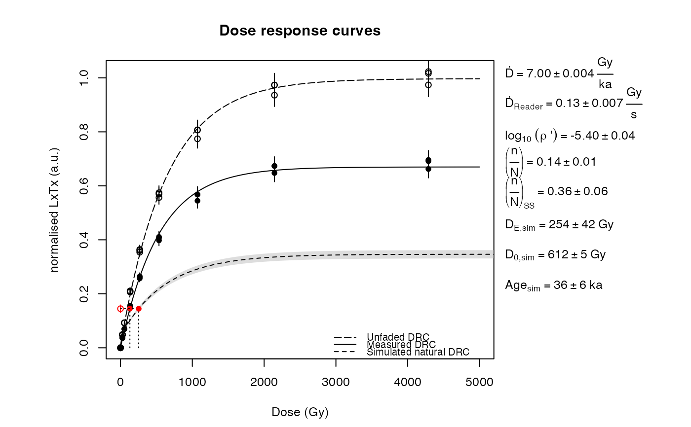
Level of saturation

The calc_Huntley2006 function also calculates the level of saturation ($\frac{n}{N}$) and the field saturation (i.e. athermal steady state, (n/N)_SS) value for the sample under investigation using the sample specific $\rho$', unfaded $D_0$ and $\dot{D}$ values, following the approach of Kars et al. (2008).

The computation is done using 1000 equally-spaced points in the interval [0.01, 3]. This can be controlled by setting option rprime, such as in rprime = seq(0.01, 3, length.out = 1000) (the default).

Uncertainties

Uncertainties are reported at $1\sigma$ and are assumed to be normally distributed and are estimated using Monte-Carlo re-sampling (n.MC = 10000 by default) of $\rho$' and $\frac{L_x}{T_x}$ during dose response curve fitting, and of $\rho$' #' in the derivation of ($n/N$) and (n/N)_SS.

Age calculated from 2D0 of the simulated natural DRC

In addition to the age calculated from the equivalent dose derived from $\frac{L_n}{T_n}$ projected on the simulated natural dose response curve (DRC), this function also calculates an age from twice the characteristic saturation dose (D0) of the simulated natural DRC. This can be a useful information for (over)saturated samples (i.e., no intersect of $\frac{L_n}{T_n}$ on the natural DRC) to obtain at least a "minimum age" estimate of the sample. In the console output this value is denoted by "Age @2D0 (ka):".

Note

This function has BETA status, in particular for the GOK implementation. Please verify your results carefully.

Function version

0.4.6

How to cite

King, G.E., Burow, C., Kreutzer, S., Colombo, M., 2025. calc_Huntley2006(): Apply the Huntley (2006) model. Function version 0.4.6. In: Kreutzer, S., Burow, C., Dietze, M., Fuchs, M.C., Schmidt, C., Fischer, M., Friedrich, J., Mercier, N., Philippe, A., Riedesel, S., Autzen, M., Mittelstrass, D., Gray, H.J., Galharret, J., Colombo, M., Steinbuch, L., Boer, A.d., 2025. Luminescence: Comprehensive Luminescence Dating Data Analysis. R package version 1.1.0. https://r-lum.github.io/Luminescence/

References

Kars, R.H., Wallinga, J., Cohen, K.M., 2008. A new approach towards anomalous fading correction for feldspar IRSL dating-tests on samples in field saturation. Radiation Measurements 43, 786-790. doi:10.1016/j.radmeas.2008.01.021

Guralnik, B., Li, B., Jain, M., Chen, R., Paris, R.B., Murray, A.S., Li, S.-H., Pagonis, P., Herman, F., 2015. Radiation-induced growth and isothermal decay of infrared-stimulated luminescence from feldspar. Radiation Measurements 81, 224-231.

Huntley, D.J., 2006. An explanation of the power-law decay of luminescence. Journal of Physics: Condensed Matter 18, 1359-1365. doi:10.1088/0953-8984/18/4/020

King, G.E., Herman, F., Lambert, R., Valla, P.G., Guralnik, B., 2016. Multi-OSL-thermochronometry of feldspar. Quaternary Geochronology 33, 76-87. doi:10.1016/j.quageo.2016.01.004

Further reading

Morthekai, P., Jain, M., Cunha, P.P., Azevedo, J.M., Singhvi, A.K., 2011. An attempt to correct for the fading in million year old basaltic rocks. Geochronometria 38(3), 223-230.

Author

Georgina E. King, University of Lausanne (Switzerland)
Christoph Burow, University of Cologne (Germany)
Sebastian Kreutzer, Institute of Geography, Heidelberg University (Germany)
Marco Colombo, Institute of Geography, Heidelberg University (Germany) , RLum Developer Team

Examples


## Load example data (sample UNIL/NB123, see ?ExampleData.Fading)
data("ExampleData.Fading", envir = environment())

## (1) Set all relevant parameters
# a. fading measurement data (IR50)
fading_data <- ExampleData.Fading$fading.data$IR50

# b. Dose response curve data
data <- ExampleData.Fading$equivalentDose.data$IR50

## (2) Define required function parameters
ddot <- c(7.00, 0.004)
readerDdot <- c(0.134, 0.0067)

# Analyse fading measurement and get an estimate of rho'.
# Note that the RLum.Results object can be directly used for further processing.
# The number of MC runs is reduced for this example
rhop <- analyse_FadingMeasurement(fading_data, plot = TRUE, verbose = FALSE, n.MC = 10)


## (3) Apply the Kars et al. (2008) model to the data
kars <- calc_Huntley2006(
 data = data,
 rhop = rhop,
 ddot = ddot,
 readerDdot = readerDdot,
 n.MC = 25)



#> 
#> 
#> [calc_Huntley2006()]
#> 
#>  -------------------------------
#>  (n/N) [-]:	 0.15 ± 0.02
#>  (n/N)_SS [-]:	 0.36 ± 0.04
#> 
#>  ---------- Measured -----------
#>  DE [Gy]:	 130.97 ± 12.87
#>  D0 [Gy]:	 539.01 ± 22.26
#>  Age [ka]:	 18.71 ± 2.06
#> 
#>  ---------- Un-faded -----------
#>  D0 [Gy]:	 638.66 ± 13.39
#> 
#>  ---------- Simulated ----------
#>  DE [Gy]:	 248.92 ± 45.16
#>  D0 [Gy]:	 611.59 ± 4.89
#>  Age [ka]:	 35.56 ± 6.69
#>  Age @2D0 [ka]:	 174.74 ± 8.85
#>  -------------------------------
#> 


if (FALSE) { # \dontrun{
# You can also provide LnTn values separately via the 'LnTn' argument.
# Note, however, that the data frame for 'data' must then NOT contain
# a LnTn value. See argument descriptions!
LnTn <- data.frame(
 LnTn = c(1.84833, 2.24833),
 nTn.error = c(0.17, 0.22))

LxTx <- data[2:nrow(data), ]

kars <- calc_Huntley2006(
 data = LxTx,
 LnTn = LnTn,
 rhop = rhop,
 ddot = ddot,
 readerDdot = readerDdot,
 n.MC = 25)
} # }