Calculate Global Standardised Growth Curve (gSGC) for Feldspar MET-pIRIR
Source:R/calc_gSGC_feldspar.R
calc_gSGC_feldspar.RdImplementation of the gSGC approach for feldspar MET-pIRIR by Li et al. (2015)
Usage
calc_gSGC_feldspar(
  data,
  gSGC.type = "50LxTx",
  gSGC.parameters = NULL,
  n.MC = 100,
  plot = FALSE
)
Arguments
- data
data.frame (required): data frame with five columns per sample
c("LnTn", "LnTn.error", "Lr1Tr1", "Lr1Tr1.error","Dr1")- gSGC.type
character (with default): growth curve type to be selected according to Table 3 in Li et al. (2015). Allowed options are
"50LxTx","50Lx","50Tx","100LxTx","100Lx","100Tx","150LxTx","150Lx","150Tx","200LxTx","200Lx","200Tx","250LxTx","250Lx","250Tx"- gSGC.parameters
data.frame (optional): an own parameter set for the gSGC with the following columns
y1,y1_err,D1D1_err,y2,y2_err,y0,y0_err.- n.MC
numeric (with default): number of Monte-Carlo runs for the error calculation
- plot
logical (with default): enable/disable the plot output.
Value
Returns an S4 object of type RLum.Results.
@data$ df (data.frame) .. $DE the calculated equivalent dose.. $DE.ERROR error on the equivalent dose, which is the standard deviation of the MC runs.. $HPD95_LOWER lower boundary of the highest probability density (95%).. $HPD95_UPPER upper boundary of the highest probability density (95%)$ m.MC (list) numeric vector with results from the MC runs.
@info
`$ call“ (call) the original function call
How to cite
Gray, H.J., Kreutzer, S., 2026. calc_gSGC_feldspar(): Calculate Global Standardised Growth Curve (gSGC) for Feldspar MET-pIRIR. Function version 0.1.1. In: Kreutzer, S., Burow, C., Dietze, M., Fuchs, M.C., Schmidt, C., Fischer, M., Friedrich, J., Mercier, N., Philippe, A., Riedesel, S., Autzen, M., Mittelstrass, D., Gray, H.J., Galharret, J., Colombo, M., Steinbuch, L., Boer, A.d., Bluszcz, A., 2026. Luminescence: Comprehensive Luminescence Dating Data Analysis. R package version 1.2.1. https://r-lum.github.io/Luminescence/
References
Li, B., Roberts, R.G., Jacobs, Z., Li, S.-H., Guo, Y.-J., 2015. Construction of a “global standardised growth curve” (gSGC) for infrared stimulated luminescence dating of K-feldspar 27, 119–130. doi:10.1016/j.quageo.2015.02.010
Author
Harrison Gray, USGS (United States), Sebastian Kreutzer, F2.1 Geophysical Parametrisation/Regionalisation, LIAG - Institute for Applied Geophysics (Germany) , RLum Developer Team
Examples
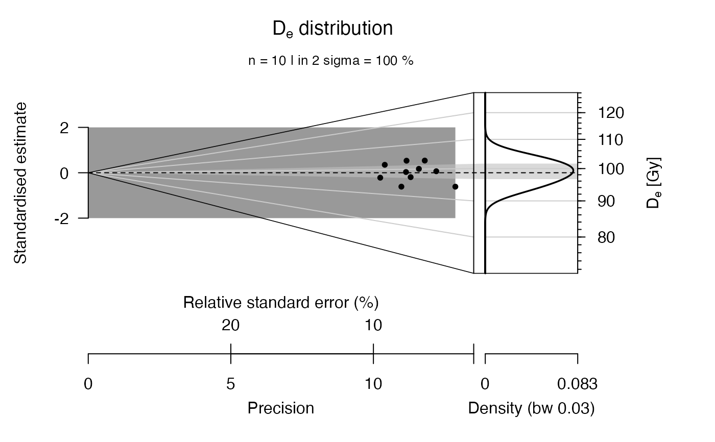
##test on a generated random sample
n_samples <- 10
data <- data.frame(
  LnTn = rnorm(n=n_samples, mean=1.0, sd=0.02),
  LnTn.error = rnorm(n=n_samples, mean=0.05, sd=0.002),
  Lr1Tr1 = rnorm(n=n_samples, mean=1.0, sd=0.02),
  Lr1Tr1.error = rnorm(n=n_samples, mean=0.05, sd=0.002),
  Dr1 = rep(100,n_samples))

results <- calc_gSGC_feldspar(
  data = data, gSGC.type = "50LxTx",
  plot = FALSE)

plot_AbanicoPlot(results)