Analyse SAR CW-OSL measurements.

The function analyses SAR CW-OSL curve data and provides a summary of the measured data for every position. The output of the function is optimised for SAR OSL measurements on quartz.

Analyse_SAR.OSLdata(
  input.data,
  signal.integral,
  background.integral,
  position,
  run,
  set,
  dtype,
  keep.SEL = FALSE,
  info.measurement = "unkown measurement",
  output.plot = FALSE,
  output.plot.single = FALSE,
  cex.global = 1,
  ...
)

Arguments

input.data: Risoe.BINfileData (required): input data from a Risø BIN file, produced by the function read_BIN2R.
signal.integral: vector (required): channels used for the signal integral, e.g. signal.integral=c(1:2)
background.integral: vector (required): channels used for the background integral, e.g. background.integral=c(85:100)
position: vector (optional): reader positions that want to be analysed (e.g. position=c(1:48). Empty positions are automatically omitted. If no value is given all positions are analysed by default.
run: vector (optional): range of runs used for the analysis. If no value is given the range of the runs in the sequence is deduced from the Risoe.BINfileData object.
set: vector (optional): range of sets used for the analysis. If no value is given the range of the sets in the sequence is deduced from the Risoe.BINfileData object.
dtype: character (optional): allows to further limit the curves by their data type (DTYPE), e.g., dtype = c("Natural", "Dose") limits the curves to this two data types. By default all values are allowed. See Risoe.BINfileData for allowed data types.
keep.SEL: logical (default): option allowing to use the SEL element of the Risoe.BINfileData manually. NOTE: In this case any limitation provided by run, set and dtype are ignored!
info.measurement: character (with default): option to provide information about the measurement on the plot output (e.g. name of the BIN or BINX file).
output.plot: logical (with default): plot output (TRUE/FALSE)
output.plot.single: logical (with default): single plot output (TRUE/FALSE) to allow for plotting the results in single plot windows. Requires output.plot = TRUE.
cex.global: numeric (with default): global scaling factor.
...: further arguments that will be passed to the function calc_OSLLxTxRatio (supported: background.count.distribution, sigmab, sig0; e.g., for instrumental error) and can be used to adjust the plot. Supported" mtext, log

Value

A plot (optional) and list is returned containing the following elements:

LnLxTnTx: data.frame of all calculated Lx/Tx values including signal, background counts and the dose points.
RejectionCriteria: data.frame with values that might by used as rejection criteria. NA is produced if no R0 dose point exists.
SARParameters: data.frame of additional measurement parameters obtained from the BIN file, e.g. preheat or read temperature (not valid for all types of measurements).

Details

The function works only for standard SAR protocol measurements introduced by Murray and Wintle (2000) with CW-OSL curves. For the calculation of the Lx/Tx value the function calc_OSLLxTxRatio is used.

Provided rejection criteria

[recyling ratio]: calculated for every repeated regeneration dose point.

[recuperation]: recuperation rate calculated by comparing the Lx/Tx values of the zero regeneration point with the Ln/Tn value (the Lx/Tx ratio of the natural signal). For methodological background see Aitken and Smith (1988)

[IRSL/BOSL]: the integrated counts (signal.integral) of an IRSL curve are compared to the integrated counts of the first regenerated dose point. It is assumed that IRSL curves got the same dose as the first regenerated dose point. Note: This is not the IR depletion ratio described by Duller (2003).

Note

Rejection criteria are calculated but not considered during the analysis to discard values.

The analysis of IRSL data is not directly supported. You may want to consider using the functions analyse_SAR.CWOSL or analyse_pIRIRSequence instead.

The development of this function will not be continued. We recommend to use the function analyse_SAR.CWOSL or instead.

Function version

0.2.17

How to cite

Kreutzer, S., Fuchs, M.C., 2023. Analyse_SAR.OSLdata(): Analyse SAR CW-OSL measurements.. Function version 0.2.17. In: Kreutzer, S., Burow, C., Dietze, M., Fuchs, M.C., Schmidt, C., Fischer, M., Friedrich, J., Mercier, N., Philippe, A., Riedesel, S., Autzen, M., Mittelstrass, D., Gray, H.J., Galharret, J., 2023. Luminescence: Comprehensive Luminescence Dating Data Analysis. R package version 0.9.23. https://CRAN.R-project.org/package=Luminescence

References

Aitken, M.J. and Smith, B.W., 1988. Optical dating: recuperation after bleaching. Quaternary Science Reviews 7, 387-393.

Duller, G., 2003. Distinguishing quartz and feldspar in single grain luminescence measurements. Radiation Measurements, 37 (2), 161-165.

Murray, A.S. and Wintle, A.G., 2000. Luminescence dating of quartz using an improved single-aliquot regenerative-dose protocol. Radiation Measurements 32, 57-73.

Author

Sebastian Kreutzer, Institute of Geography, Heidelberg University (Germany)
Margret C. Fuchs, HZDR, Freiberg (Germany) , RLum Developer Team

Examples

##load data
data(ExampleData.BINfileData, envir = environment())

##analyse data
output <- Analyse_SAR.OSLdata(input.data = CWOSL.SAR.Data,
                              signal.integral = c(1:5),
                              background.integral = c(900:1000),
                              position = c(1:1),
                              output.plot = TRUE)

#> 
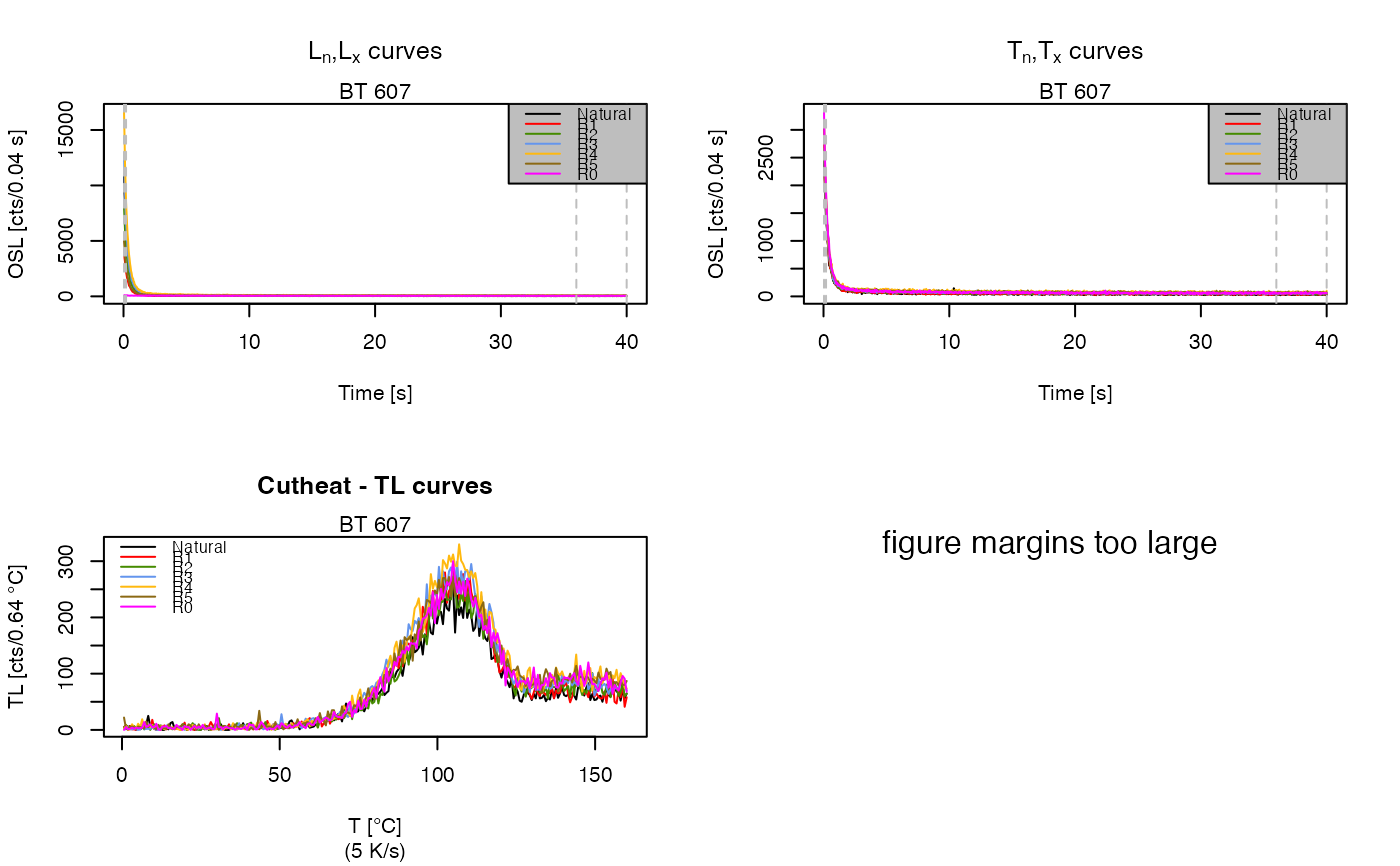#> [Analyse_SAR.OSLdata()] >> Figure for position 1 produced.

##combine results relevant for further analysis
output.SAR <- data.frame(Dose = output$LnLxTnTx[[1]]$Dose,
                         LxTx = output$LnLxTnTx[[1]]$LxTx,
                         LxTx.Error = output$LnLxTnTx[[1]]$LxTx.Error)
output.SAR
#>   Dose       LxTx  LxTx.Error
#> 1    0 4.31385656 0.049585512
#> 2  450 1.54110507 0.020078494
#> 3 1050 3.03229838 0.035808499
#> 4 2000 4.59447529 0.050759620
#> 5 2550 5.31012713 0.054631294
#> 6  450 1.61167200 0.019431239
#> 7    0 0.01668642 0.001735488