Apply the finite mixture model (FMM) after Galbraith (2005) to a given De distribution
Source:R/calc_FiniteMixture.R
calc_FiniteMixture.RdThis function fits a k-component mixture to a De distribution with differing known standard errors. Parameters (doses and mixing proportions) are estimated by maximum likelihood assuming that the log dose estimates come from a mixture of normal distributions.
Arguments
- data
RLum.Results or data.frame (required): for data.frame: two columns with De
(data[,1])and De error(values[,2])- sigmab
numeric (required): spread in De values (given as a fraction, e.g. 0.2), representing the expected overdispersion in the data should the sample be well-bleached (Cunningham & Wallinga 2012, p. 100).
- n.components
numeric (required): number of components to be fitted. If a vector is provided (e.g.
c(2:8)) the finite mixtures for 2, 3 ... 8 components are calculated and a plot and a statistical evaluation of the model performance (BIC score and maximum log-likelihood) is provided.- grain.probability
logical (with default): prints the estimated probabilities of which component each grain is in
- pdf.weight
logical (with default): weight the probability density functions by the components proportion. Ignored if
n.componentshas length 1.- pdf.sigma
character (with default): if
"sigmab"the components normal distributions are plotted with a common standard deviation (i.e.sigmab) as assumed by the FFM. Alternatively,"se"takes the standard error of each component for the sigma parameter of the normal distribution- pdf.colors
character (with default): colour coding of the components in the plot. Possible options are
"gray","colors"and"none".- plot.proportions
logical (with default): plot a graphics::barplot showing the proportions of components. Ignored if
n.componentshas length 1.- plot.criteria
logical (with default): plot the statistical criteria (BIC and log-likelihood). Ignored if
n.componentshas length 1.- plot
logical (with default): enable/disable the plot output. This is ignored and no plot is produced if
n.componentshas length 1.- ...
other parameters to control the plot output. Supported are
cex,main,main.densities,main.proportions,main.criteria,pdf.scale,dose.scale.
Value
Returns a plot (optional) and terminal output. In addition an RLum.Results object is returned containing the following elements:
- .$summary
data.frame summary of all relevant model results.
- .$data
data.frame original input data
- .$args
list used arguments
- .$call
call the function call
- .$mle
covariance matrices of the log likelihoods
- .$BIC
BIC score
- .$llik
maximum log likelihood
- .$grain.probability
probabilities of a grain belonging to a component
- .$components
matrix estimates of the de, de error and proportion for each component
- .$single.comp
data.frame single component FFM estimate
If a vector for n.components is provided (e.g. c(2:8)),
mle and grain.probability are lists containing matrices of the
results for each iteration of the model.
The output should be accessed using the function get_RLum.
Details
This model uses the maximum likelihood and Bayesian Information Criterion (BIC) approaches.
Indications of overfitting are:
increasing BIC
repeated dose estimates
covariance matrix not positive definite
covariance matrix produces
NaNconvergence problems
Plot
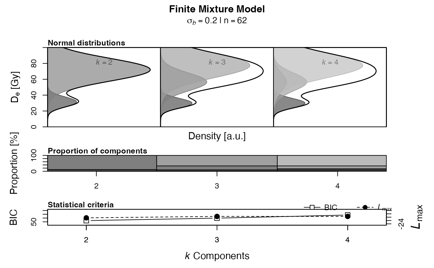
If n.components is a vector (c(k.min:k.max)), a plot is generated
showing the k components equivalent doses as normal distributions.
By default pdf.weight is set to TRUE, so that the probability density
functions are weighted by the components proportion for each iteration of
k components, so the sum of areas of each component equals 1.
If pdf.weight is set to FALSE, the area under each normal distribution
is always 1. While the density values are on the same scale when no weights
are used, the y-axis are individually scaled if the probability density are
weighted by the components proportion.
The standard deviation (sigma) of the normal distributions is by default
determined by a common sigmab (see pdf.sigma). For
pdf.sigma = "se" the standard error of each component is taken
instead.
The stacked graphics::barplot shows the proportion of each component (in
per cent) calculated by the FMM. The last plot shows the achieved BIC scores
and maximum log-likelihood estimates for each value of k.
How to cite
Burow, C., Colombo, M., 2026. calc_FiniteMixture(): Apply the finite mixture model (FMM) after Galbraith (2005) to a given De distribution. Function version 0.4.4. In: Kreutzer, S., Burow, C., Dietze, M., Fuchs, M.C., Schmidt, C., Fischer, M., Friedrich, J., Mercier, N., Philippe, A., Riedesel, S., Autzen, M., Mittelstrass, D., Gray, H.J., Galharret, J., Colombo, M., Steinbuch, L., Boer, A.d., Bluszcz, A., 2026. Luminescence: Comprehensive Luminescence Dating Data Analysis. R package version 1.3.0. https://r-lum.github.io/Luminescence/
References
Galbraith, R.F. & Green, P.F., 1990. Estimating the component ages in a finite mixture. Nuclear Tracks and Radiation Measurements 17, 197-206.
Galbraith, R.F. & Laslett, G.M., 1993. Statistical models for mixed fission track ages. Nuclear Tracks Radiation Measurements 4, 459-470.
Galbraith, R.F. & Roberts, R.G., 2012. Statistical aspects of equivalent dose and error calculation and display in OSL dating: An overview and some recommendations. Quaternary Geochronology 11, 1-27.
Roberts, R.G., Galbraith, R.F., Yoshida, H., Laslett, G.M. & Olley, J.M., 2000. Distinguishing dose populations in sediment mixtures: a test of single-grain optical dating procedures using mixtures of laboratory-dosed quartz. Radiation Measurements 32, 459-465.
Galbraith, R.F., 2005. Statistics for Fission Track Analysis, Chapman & Hall/CRC, Boca Raton.
Further reading
Arnold, L.J. & Roberts, R.G., 2009. Stochastic modelling of multi-grain equivalent dose (De) distributions: Implications for OSL dating of sediment mixtures. Quaternary Geochronology 4, 204-230.
Cunningham, A.C. & Wallinga, J., 2012. Realizing the potential of fluvial archives using robust OSL chronologies. Quaternary Geochronology 12, 98-106.
Rodnight, H., Duller, G.A.T., Wintle, A.G. & Tooth, S., 2006. Assessing the reproducibility and accuracy of optical dating of fluvial deposits. Quaternary Geochronology 1, 109-120.
Rodnight, H. 2008. How many equivalent dose values are needed to obtain a reproducible distribution?. Ancient TL 26, 3-10.
Author
Christoph Burow, University of Cologne (Germany)
Marco Colombo, Institute of Geography, Heidelberg University (Germany)
Based on a rewritten S script of Rex Galbraith, 2006.
, RLum Developer Team
Examples
## load example data
data(ExampleData.DeValues, envir = environment())

## (1) apply the finite mixture model
## NOTE: the data set is not suitable for the finite mixture model,
## which is why a very small sigmab is necessary
calc_FiniteMixture(ExampleData.DeValues$CA1,
                   sigmab = 0.2, n.components = 2,
                   grain.probability = TRUE)
#>
#>  [calc_FiniteMixture]
#>
#> ----------- meta data ------------
#>  n:                     62
#>  sigmab:                0.2
#>  number of components:  2
#>  llik:                  -20.3938
#>  BIC:                   53.169
#>
#> --- covariance matrix of mle's ---
#>
#>          [,1]     [,2]     [,3]
#> [1,] 0.002144 0.001821 0.000283
#> [2,] 0.001821 0.013319 0.000877
#> [3,] 0.000283 0.000877 0.001118
#>
#>
#> ----------- components -----------
#>
#>                 comp1   comp2
#>
#> dose (Gy)     31.5299 72.0333
#> rse(dose)      0.1154  0.0334
#> se(dose)(Gy)   3.6387  2.4082
#>
#> proportion     0.1096  0.8904
#>
#> -------- grain probability -------
#>
#>       [,1] [,2]
#>  [1,] 1.00 0.00
#>  [2,] 1.00 0.00
#>  [3,] 1.00 0.00
#>  [4,] 0.99 0.01
#>  [5,] 0.94 0.06
#>  [6,] 0.91 0.09
#>  [7,] 0.29 0.71
#>  [8,] 0.13 0.87
#>  [9,] 0.11 0.89
#> [10,] 0.10 0.90
#> [11,] 0.09 0.91
#> [12,] 0.06 0.94
#> [13,] 0.04 0.96
#> [14,] 0.03 0.97
#> [15,] 0.04 0.96
#> [16,] 0.02 0.98
#> [17,] 0.01 0.99
#> [18,] 0.01 0.99
#> [19,] 0.01 0.99
#> [20,] 0.00 1.00
#> [21,] 0.00 1.00
#> [22,] 0.00 1.00
#> [23,] 0.00 1.00
#> [24,] 0.00 1.00
#> [25,] 0.00 1.00
#> [26,] 0.00 1.00
#> [27,] 0.00 1.00
#> [28,] 0.00 1.00
#> [29,] 0.00 1.00
#> [30,] 0.00 1.00
#> [31,] 0.00 1.00
#> [32,] 0.00 1.00
#> [33,] 0.00 1.00
#> [34,] 0.00 1.00
#> [35,] 0.00 1.00
#> [36,] 0.00 1.00
#> [37,] 0.00 1.00
#> [38,] 0.00 1.00
#> [39,] 0.00 1.00
#> [40,] 0.00 1.00
#> [41,] 0.00 1.00
#> [42,] 0.00 1.00
#> [43,] 0.00 1.00
#> [44,] 0.00 1.00
#> [45,] 0.00 1.00
#> [46,] 0.00 1.00
#> [47,] 0.00 1.00
#> [48,] 0.00 1.00
#> [49,] 0.00 1.00
#> [50,] 0.00 1.00
#> [51,] 0.00 1.00
#> [52,] 0.00 1.00
#> [53,] 0.00 1.00
#> [54,] 0.00 1.00
#> [55,] 0.00 1.00
#> [56,] 0.00 1.00
#> [57,] 0.00 1.00
#> [58,] 0.00 1.00
#> [59,] 0.00 1.00
#> [60,] 0.00 1.00
#> [61,] 0.00 1.00
#> [62,] 0.00 1.00
#>
#>
#> -------- single component --------
#>  mu:                     65.2273
#>  sigmab:                 0.2
#>  llik:                   -44.96
#>  BIC:                    94.047
#>
#> [calc_FiniteMixture()] 'n.components' specified only one component, nothing plotted

## (2) repeat the finite mixture model for 2, 3 and 4 maximum number of fitted
## components and save results
## NOTE: The following example is computationally intensive. Please un-comment
## the following lines to make the example work.
FMM<- calc_FiniteMixture(ExampleData.DeValues$CA1,
                         sigmab = 0.2, n.components = c(2:4),
                         pdf.weight = TRUE)
#>
#>  [calc_FiniteMixture]
#>
#> ----------- meta data ------------
#>  n:                     62
#>  sigmab:                0.2
#>  number of components:  2, 3, 4
#>
#> -------- single component --------
#>  mu:                     65.2273
#>  sigmab:                 0.2
#>  llik:                   -44.96
#>  BIC:                    94.047
#>
#>
#> ---------- k components ----------
#>             2     3     4
#> c1_dose 31.53 29.91 29.91
#> c1_se    3.64  3.97  4.32
#> c1_prop  0.11  0.09  0.09
#> c2_dose 72.03 56.65 56.65
#> c2_se    2.41 13.05 33.16
#> c2_prop  0.89  0.25  0.07
#> c3_dose  <NA> 77.49 56.65
#> c3_se    <NA>  6.37 21.31
#> c3_prop  <NA>  0.66  0.18
#> c4_dose  <NA>  <NA> 77.49
#> c4_se    <NA>  <NA>  7.68
#> c4_prop  <NA>  <NA>  0.66
#>
#> ------ statistical criteria ------
#>             1       2       3       4
#> BIC    94.047  53.169  59.719  67.973
#> loglik -44.96 -20.394 -19.542 -19.542
#> signif            ***
#>
#>  Lowest BIC score for k = 2
#>  First significant increase in maximum log-likelihood for k = 2
#>


## show structure of the results
FMM
#>
#>  [RLum.Results-class]
#> 	 originator: calc_FiniteMixture()
#> 	 data: 10
#>  	 .. $summary : data.frame
#> 	 .. $data : data.frame
#> 	 .. $args : list
#> 	 .. $call : call
#> 	 .. $mle : list
#> 	 .. $BIC : data.frame
#> 	 .. $llik : data.frame
#> 	 .. $grain.probability : list
#> 	 .. $components : matrix
#> 	 .. $single.comp : data.frame
#> 	 additional info elements:  0

## show the results on equivalent dose, standard error and proportion of
## fitted components
get_RLum(object = FMM, data.object = "components")
#>               2       3       4
#> c1_dose 31.5299 29.9146 29.9147
#> c1_se    3.6387  3.9695  4.3219
#> c1_prop  0.1096  0.0891  0.0891
#> c2_dose 72.0333 56.6455 56.6458
#> c2_se    2.4082 13.0496 33.1629
#> c2_prop  0.8904  0.2480  0.0725
#> c3_dose      NA 77.4938 56.6458
#> c3_se        NA  6.3696 21.3092
#> c3_prop      NA  0.6629  0.1755
#> c4_dose      NA      NA 77.4940
#> c4_se        NA      NA  7.6758
#> c4_prop      NA      NA  0.6629
## show structure of the results
FMM
#>
#> [RLum.Results-class]
#> originator: calc_FiniteMixture()
#> data: 10
#> .. $summary : data.frame
#> .. $data : data.frame
#> .. $args : list
#> .. $call : call
#> .. $mle : list
#> .. $BIC : data.frame
#> .. $llik : data.frame
#> .. $grain.probability : list
#> .. $components : matrix
#> .. $single.comp : data.frame
#> additional info elements: 0
## show the results on equivalent dose, standard error and proportion of
## fitted components
get_RLum(object = FMM, data.object = "components")
#> 2 3 4
#> c1_dose 31.5299 29.9146 29.9147
#> c1_se 3.6387 3.9695 4.3219
#> c1_prop 0.1096 0.0891 0.0891
#> c2_dose 72.0333 56.6455 56.6458
#> c2_se 2.4082 13.0496 33.1629
#> c2_prop 0.8904 0.2480 0.0725
#> c3_dose NA 77.4938 56.6458
#> c3_se NA 6.3696 21.3092
#> c3_prop NA 0.6629 0.1755
#> c4_dose NA NA 77.4940
#> c4_se NA NA 7.6758
#> c4_prop NA NA 0.6629