This function applies the fading correction for the prediction of long-term fading as suggested by Lamothe et al., 2003. The function basically adjusts the $L_n/T_n$ values and fits a new dose-response curve using function fit_DoseResponseCurve.
Usage
calc_Lamothe2003(
  object,
  dose_rate.envir,
  dose_rate.source,
  g_value,
  tc = NULL,
  tc.g_value = tc,
  verbose = TRUE,
  plot = TRUE,
  ...
)
Arguments
- object
RLum.Results data.frame (required): Input data for applying the fading correction, can be (1) a data.frame with three columns (
dose,LxTx,LxTx error; see details), or (2) an RLum.Results object created by analyse_SAR.CWOSL or analyse_pIRIRSequence.- dose_rate.envir
numeric vector of length 2 (required): Environmental dose rate in mGy/a.
- dose_rate.source
numeric vector of length 2 (required): Irradiation source dose rate in Gy/s, which is, according to Lamothe et al. (2003) De/t.
- g_value
numeric vector of length 2 (required): g_value in %/decade recalculated at the moment the equivalent dose was calculated, i.e.
tcis either similar for the g-value measurement and the De measurement or needs be to recalculated (cf. calc_FadingCorr). Inserting a normalised g-value, e.g., normalised to 2-days , will lead to wrong results.- tc
numeric (optional): time in seconds between the end of the irradiation and the prompt measurement used in the equivalent dose estimation (cf. Huntley & Lamothe 2001). If set to
NULL, it is assumed thattcis similar for the equivalent dose estimation and the g-value estimation.- tc.g_value
numeric (with default): time in seconds between irradiation and the prompt measurement estimating the g-value. If the g-value was normalised to, e.g., 2 days, this time in seconds (i.e.,
172800) should be entered here along with the time used for the equivalent dose estimation. If nothing is provided the time is set totc, which is the usual case for g-values obtained using the SAR method and g-values that had been not normalised to 2 days. Note: If this value is notNULLthe functions expects a numeric value fortc.- verbose
logical (with default): enable/disable output to the terminal.
- plot
logical (with default): enable/disable the plot output.
- ...
further arguments passed to plot_DoseResponseCurve.
Value
The function returns an RLum.Results object and the graphical output produced by plot_DoseResponseCurve.
———————————–[ NUMERICAL OUTPUT ]
———————————–
RLum.Results-object
slot: @data
| Element | Type | Description |
$data | data.frame | the fading corrected values |
$fit | nls | the object returned by the dose response curve fitting |
'slot: @info
The original function call
Details
Format of object if data.frame
If object is a data.frame, all input values must be of type numeric.
Dose values are expected in seconds (s) not Gray (Gy). No NA values are
allowed and the value for the natural dose (first row) should be 0.
Example for three dose points (column names are arbitrary):
Note on the g-value and tc
Users new to R and fading measurements are often confused about what to
enter for tc and why it may differ from tc.g_value. By convention
(Huntley & Lamothe 2001), the tc value is the time elapsed between the
end of the irradiation and the prompt measurement. Usually there is no
reason for having a tc value different for the equivalent dose measurement
and the g-value measurement, except if different equipment was used.
However, if, for instance, the g-value measurement sequence was analysed
with the Analyst (Duller 2015) and Luminescence is used to correct for
fading, there is a high chance that the value returned by the Analyst
comes normalised to 2-days, even if the tc values of the measurement were
identical. In such cases, the fading correction cannot be correct until the
tc.g_value is manually set to 2-days (172800 s) because the function
will internally recalculate values to an identical tc value.
How to cite
Kreutzer, S., Mercier, N., 2026. calc_Lamothe2003(): Apply fading correction after Lamothe et al., 2003. Function version 0.1.1. In: Kreutzer, S., Burow, C., Dietze, M., Fuchs, M.C., Schmidt, C., Fischer, M., Friedrich, J., Mercier, N., Philippe, A., Riedesel, S., Autzen, M., Mittelstrass, D., Gray, H.J., Galharret, J., Colombo, M., Steinbuch, L., Boer, A.d., Bluszcz, A., 2026. Luminescence: Comprehensive Luminescence Dating Data Analysis. R package version 1.2.1. https://r-lum.github.io/Luminescence/
References
Huntley, D.J., Lamothe, M., 2001. Ubiquity of anomalous fading in K-feldspars and the measurement and correction for it in optical dating. Canadian Journal of Earth Sciences 38, 1093-1106.
Duller, G.A.T., 2015. The Analyst software package for luminescence data: overview and recent improvements. Ancient TL 33, 35–42.
Lamothe, M., Auclair, M., Hamzaoui, C., Huot, S., 2003. Towards a prediction of long-term anomalous fading of feldspar IRSL. Radiation Measurements 37, 493-498.
Author
Sebastian Kreutzer, F2.1 Geophysical Parametrisation/Regionalisation, LIAG - Institute for Applied Geophysics (Germany)
Norbert Mercier, IRAMAT-CRP2A, Université Bordeaux Montaigne (France)
, RLum Developer Team
Examples
##load data
##ExampleData.BINfileData contains two BINfileData objects
##CWOSL.SAR.Data and TL.SAR.Data
data(ExampleData.BINfileData, envir = environment())
##transform the values from the first position in a RLum.Analysis object
object <- Risoe.BINfileData2RLum.Analysis(CWOSL.SAR.Data, pos=1)
##perform SAR analysis and set rejection criteria
results <- analyse_SAR.CWOSL(
object = object,
signal_integral = 1:2,
background_integral = 900:900,
verbose = FALSE,
plot = FALSE,
onlyLxTxTable = TRUE
)
#> Warning: [analyse_SAR.CWOSL()] Background integral should contain at least two values, reset to 875:900
##run fading correction
results_corr <- calc_Lamothe2003(
object = results,
dose_rate.envir = c(1.676 , 0.180),
dose_rate.source = c(0.184, 0.003),
g_value = c(2.36, 0.6),
plot = TRUE,
fit.method = "EXP")
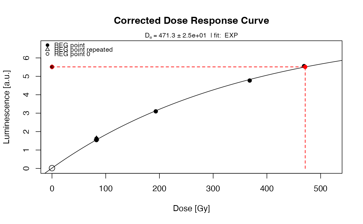 #>
#> [calc_Lamothe2003()]
#>
#> Used g_value: 2.36 ± 0.6 %/decade
#>
#> Fading_C: 0.785 ± 0.055
#> Corrected Ln/Tn: 5.515 ± 0.391
#> Corrected De: 472.55 ± 65.38 Gy
#> --------------------------------------------------------
#> Corrected Age: 281.95 ± 49.38 ka
#> --------------------------------------------------------
#>
#> [calc_Lamothe2003()]
#>
#> Used g_value: 2.36 ± 0.6 %/decade
#>
#> Fading_C: 0.785 ± 0.055
#> Corrected Ln/Tn: 5.515 ± 0.391
#> Corrected De: 472.55 ± 65.38 Gy
#> --------------------------------------------------------
#> Corrected Age: 281.95 ± 49.38 ka
#> --------------------------------------------------------